Foundation 施工笔记【6】- 路径追踪

Preface

Foundation现在(2025/12/16)也有了能用的RT相关API，Editor的GPUScene也有了BLAS上传/压缩(compact)与逐帧TLAS更新支持。到目前为止用rt做的只有inline query实现硬阴影——在做实时GI相关内容之前，不妨复习下采样/PBR相关知识——那就写个GPU Path Tracer吧？

PBRT/Physically Based Rendering:From Theory To Implementation/Kanition大佬v3翻译版，Ray Tracing Gems 2, nvpro-samples/vk_gltf_renderer 将是我们这里主要的信息来源。

准备工作

SBT (Shader Binding Table) 及管线 API

之前用过了非常方便的Inline Ray Query - 从fragment/pixel，compute可以直接产生光线进行trace：从这里出发进行PT是可行的，这也是nvpro-samples/vk_mini_path_tracer 的教学式做法。

不过完全利用硬件的RT管线会离不开SBT/Shader Binding Table，即Shader绑定表。除了shader单体更小更快之外，调度也有由驱动优化的可能。

实现上…初见确实给了不少震撼。庆幸自己选择了去写个RHI，不然Vulkan SBT方面API的繁文缛节实在是难受- -

保持不特化shader（即shader内各种魔法宏 - 点名Unity，UE）的原则，以下是最后实践的shader绑定API。此外，整个路径追踪过程的C++部分也在此一览无余。

renderer->CreatePass(
    "Trace", RHIDeviceQueueType::Graphics, 0u,
    [=](PassHandle self, Renderer* r)
    {
        r->BindBufferUniform(self, GlobalUBO, RHIPipelineStageBits::RayTracingShader, "globalParams");
        r->BindAccelerationStructureSRV(self, TLAS, RHIPipelineStageBits::RayTracingShader, "AS");
        r->BindShader(self, RHIShaderStageBits::RayGeneration, "RayGeneration", "data/shaders/ERTPathTracer.spv",
                      AsBytes(AsSpan(cfg.viewFlags)));
        r->BindShader(self, RHIShaderStageBits::RayClosestHit, "RayClosestHit", "data/shaders/ERTPathTracer.spv",
                      AsBytes(AsSpan(cfg.viewFlags)), /*hit group*/ 0);
        r->BindShader(self, RHIShaderStageBits::RayAnyHit, "RayOpacityAnyHit", "data/shaders/ERTPathTracer.spv",
          AsBytes(AsSpan(cfg.viewFlags)), /*hit group*/ 0);
        r->BindShader(self, RHIShaderStageBits::RayMiss, "RayMiss", "data/shaders/ERTPathTracer.spv",
                      AsBytes(AsSpan(cfg.viewFlags)));
        r->BindShader(self, RHIShaderStageBits::RayAnyHit, "ShadowRayAnyHit", "data/shaders/ERTPathTracer.spv",
                      AsBytes(AsSpan(cfg.viewFlags)), /*hit group*/ 1);
        r->BindShader(self, RHIShaderStageBits::RayMiss, "ShadowRayMiss", "data/shaders/ERTPathTracer.spv",
                      AsBytes(AsSpan(cfg.viewFlags)));
        r->BindBufferStorageRead(self, InstanceBuffer, RHIPipelineStageBits::ComputeShader, "instances");
        r->BindBufferStorageRead(self, PrimitiveBuffer, RHIPipelineStageBits::AllGraphics, "primitives");
        r->BindBufferStorageRead(self, MaterialBuffer, RHIPipelineStageBits::AllGraphics, "materials");
        r->BindTextureSampler(self, TexSampler, "textureSampler");
        r->BindDescriptorSet(self, "textures", gpu->GetTexturePool()->GetDescriptorSetLayout());
        r->BindTextureUAV(self, AccumulatedBuffer, "accumulation", RHIPipelineStageBits::RayTracingShader,
                          RHITextureViewDesc{.format = RHIResourceFormat::R16G16B16A16SignedFloat,
                                             .range = RHITextureSubresourceRange::Create()});

    }, [=](PassHandle self, Renderer* r, RHICommandList* cmd)
    {
        RHIExtent2D wh = r->GetSwapchainExtent();
        r->CmdSetPipeline(self, cmd);
        r->CmdBindDescriptorSet(self, cmd, "textures", gpu->GetTexturePool()->GetDescriptorSet());
        cmd->TraceRays(wh.x, wh.y, 1);
    });

随机数生成及采样

参考 Ray Tracing Gems 2 的 Reference Path Tracer - 随机数生成使用了书中介绍的 PCG4；参考实现中有个很有趣的hack，从uint32直接产生$[0,1)$区间的浮点数：这里贴出来。

// Converts unsigned integer into float int range <0; 1) by using 23 most significant bits for mantissa
float uintToFloat(uint x) {
	return asfloat(0x3f800000 | (x >> 9)) - 1.0f;
}

下面PT本身做的蒙特卡洛和各种重要性采样之外，Viewport采样也值得一提——产生图像的并非逐帧刷新，而存在积累过程。

毕竟，我们的随机数种子也是由帧序号初始化的——这样做可以将多帧，可能不同但趋近最终积分的结过积累以逼近。小记积累部分的更新：

float4 output = float4(L, 1.0f);
float frameCount = float(globalParams.ptAccumualatedFrames + 1);
if (frameCount == 1){
    accumulation[pix] = lighting[pix] = output;
} else {
    accumulation[pix] += output;
    lighting[pix] = accumulation[pix] / frameCount;
}

还有一个好处是：因为是多帧平均采样，若对镜头做jitter，这里就是一种 ~~五毛钱~~ TAA/Temporal抗锯齿的实现。Primiary Ray生成如下：

float3 GeneratePrimaryRay(uint2 pixel, PCG rng)
{
    float2 jitter = lerp(float2(-0.5f), float2(0.5f), float2(rng.sample(), rng.sample()));
    float2 uv = float2(pixel + jitter + 0.5f) / DispatchRaysDimensions().xy;
    float4 ndcPosition = float4(uv, 1.0f, 1.0f);
    ndcPosition.y = 1 - ndcPosition.y;
    ndcPosition.xy = ndcPosition.xy * 2.0f - 1.0f;
    float4 wsPosition = mul(globalParams.inverseViewProj, ndcPosition);
    return normalize(wsPosition.xyz / wsPosition.w - globalParams.camPosition);
}

BxDF

重头戏。~~只会复制粘贴公式可使不得（喂）~~

接下来的实现以PBRT的风格完成，以下将给出的结构及界面将同PBRT书中定义一致。此外，自己将尽力给出以下模型的原理推导。

最后作为参考，还请参阅 PBRT v4 - 9 Reflection Models 以获取最权威信息；此外，这一部分在Kanition PBRT v3翻译版中尚未完成，自己尝试的翻译和数学解释也许不够准确——如有错误还烦请指正！

漫反射（朗伯反射）

最简单的漫反射BRDF，也就是朗伯反射（Lambertian Diffuse）。图源Kanition翻译PBRTv3

他的BRDF Lobe很简单：分布是一个半球面，而且能量均匀。我们从评估/Eval（已知入射出射方向）和采样/Sample（已知出射/相机入射未知）两个方向解读 PBRT 的实现。

f/Eval

回顾渲染公式： $$ L_o(\mathbf{x}, \omega_o) = \int_{\Omega} f_r(\mathbf{x}, \omega_i, \omega_o) L_i(\mathbf{x}, \omega_i) \cos\theta ,d\omega_i $$ 朗伯反射的能量分布是无条件均匀的，那么设$f_r = kR$ 。保证能量守恒，$L_i = 1$积分有 $$ L_o = \int_{H^2}{kR cos\theta d w_i} = kR \int_{H^2}{cos\theta d w_i} = R \newline k = \frac{1}{\int_{H^2}{cos\theta d w_i}} = \frac{1}{\pi} $$

即 $f_r = \frac{R}{\pi}$，对应PBRT界面中的f()实现。

Sample_f/Sample

PBRT中使用了SampleCosineHemisphere做重要性采样（如图），采样单位圆内点后直接投影在单位球面上。

public float3 SampleCosineHemisphere(float2 u) {
    float2 d = SampleConcentricDisk(u);
    float z = SafeSqrt(1.0 - Sqr(d.x) - Sqr(d.y));
    return float3(d.x, d.y, z);
}

采样PDF推导也很直接；这里$x^2 + y^2 + z^2 = 1$，若记ConcentricDisk上极坐标为$(r, \phi)$,最后单位球坐标为$(1, \theta, \phi)$则代入：

$$ x^2 + y^2 = r^2 \newline z^2 = 1 - r^2 = cos^2{\theta} \newline sin^2\theta = r^2 \newline $$

我们有$sin \theta = r$, 接下来求变换$(r,\phi) \to (\theta,\phi)$的雅可比行列式：

$$ J = \left|\frac{\partial(r, \phi)}{\partial(\theta, \phi)}\right |= \begin{vmatrix} \cos\theta & 0 \newline 0 & 1 \end{vmatrix} = \cos\theta $$

我们知道圆盘上采样的PDF是 $ \frac{r}{\pi} $ 那么知道行列式后我们可以很轻松地得到该采样方式的PDF为 $ cos\theta \frac{r}{\pi} = \frac{cos\theta sin\theta}{\pi} $ 这里的“权重”，$cos\theta$，也正是该采样方法名字/Cosine Weighted的来源。

注意PDF对应球面上的立体角/solid angle，即$dw = sin\theta d\theta d\phi$；这里的$sin\theta$消掉，即得到我们最后采样的PDF

public float CosineHemispherePDF(float cosTheta) {
    return cosTheta * InvPi;
}

IBxDF 实现

整理完毕如下。这里（和以后的）的IBxDF界面和PBRT书中介绍将保证完全一致。

public struct DiffuseBxDF : IBxDF {
    SampledSpectrum R;
    public __init(SampledSpectrum R) {
        this.R = R;
    }
    public BxDFFlags Flags(){
        return BxDFFlags::DiffuseReflection;
    }
    // BRDF evaluation
    // Constant reflection distribution where:
    // \int_H^2 f(wo,wi) CosTheta(wi) dwi = R
    public SampledSpectrum f(float3 wo, float3 wi, TransportMode) {
        if (!SameHemisphere(wo, wi)) {
            return float3(0.0, 0.0, 0.0);
        }
        return R * InvPi;
    }
    // Draw a sample from cosine-weighted hemisphere
    public BSDFSample Sample_f(float3 wo, float uc, float2 u,TransportMode, BxDFReflTransFlags flags) {
        if (!(flags & BxDFReflTransFlags::Reflection))
            return BSDFSample();
        float3 wi = SampleCosineHemisphere(u);
        if (wo.z < 0.0) wi.z *= -1.0; // Ensure same hemisphere
        float pdf = CosineHemispherePDF(AbsCosTheta(wi));
        return BSDFSample(R * InvPi, wi, pdf, BxDFFlags::DiffuseReflection);
    }
    // Evaluated PDF for a pair of directions
    public float PDF(float3 wo, float3 wi,TransportMode, BxDFReflTransFlags flags) {
        if (!(flags & BxDFReflTransFlags::Reflection) || !SameHemisphere(wo, wi))
            return 0.0;
        return CosineHemispherePDF(AbsCosTheta(wi));
    }
};

镜面反射（完美反射）

完美的镜面反射的BRDF Lobe是个“光线”——他的分布在且仅在一个单独方向上。这可以用狄拉克$\delta$函数表达：

$$ \int f(x), \delta(x - x_0), \mathrm{d}x = f(x_0) $$ 而在BRDF中积分后，渲染等式的以下恒等关系是应该成立的：出射能量等同$入射能量*菲涅耳反射量$ $$ L_o(\omega_o) = \int_{H^2(\mathbf{n})} f_r(\omega_o, \omega_i), L_i(\omega_i), \lvert \cos \theta_i \rvert, \mathrm{d}\omega_i = F_r(\omega_r), L_i(\omega_r) $$ 一个直觉的想法就是直接用狄拉克表达$f_r$。但是这样积分完后会多出一个 $cos \theta_r$： $$ f_r(\omega_o, \omega_i) = \delta(\omega_i - \omega_r), F_r(\omega_i) \newline L_o(\omega_o) = \int_{H^2(\mathbf{n})} \delta(\omega_i - \omega_r), F_r(\omega_i), L_i(\omega_i), \lvert \cos \theta_i \rvert, \mathrm{d}\omega_i = F_r(\omega_r), L_i(\omega_r), \lvert \cos \theta_r \rvert $$ …那么一个更直觉的做法就是把这个常数拆出来：要记得我们的反射方向是已知量。最后得到镜面BRDF的最终形式： $$ f_r(\omega_o, \omega_i) = F_r(w_r)\frac{\delta(w_i-w_r)}{|cos\theta_r|} $$

f/Eval

BRDF已经给出来了。不过处理他的PDF很棘手：这里是为了镜面反射情况（roughness=0或很小）下的分布：回顾之前的Lobe图案，他只在唯一一个完美反射的方向有信号。

PDF的表达将很困难。该情况概率本身是个狄拉克$\delta$函数：全域除原点都为$0$，而积分是$1$。那么PDF在该点上则会是无穷大！

PBRT在这里对所有方向姑且直接返回$0$。应为单点真去表达的话，你会得到一个无穷亮的像素（firefly）！

Sample_f/Sample

出射向量是易知的。我们在本地切空间计算，那么$n(0,0,1)$，$w_o(x,y,z)$围绕他的反射向量很简单，Reflect()后就是$w_r(-x,-y,z)$

注：PBRT中的Reflect(v,n)和HLSL/GLSL中的Reflect(v,n)不一样：

public float3 Reflect(float3 wo, float3 n) {
    //     vvv wo is flipped (pointing away)
    return -wo + 2 * dot(wo, n) * n;
}

GLSL/HLSL中为

genType reflect(genType I, genType N);
---
For a given incident vector I and surface normal N reflect returns the reflection direction calculated as I - 2.0 * dot(N, I) * N.

他的“入射”向量是翻转的：理由嘛，就是我们在PBRT建模光路时是习惯从相机到入射的“反向”。

最后，他的PDF仍旧是个狄拉克。但是采样积分继续用$0$表示会很难受：蒙特卡洛会除以这个PDF。PBRT在此规定让狄拉克PDF在采样中的值一直为$1$。

IBxDF 实现

没有，也不必要——这里的式子会在后面设计反射的BxDF反复利用…接下来介绍当反射面并非“完美”，而带粗糙度的情况。

Microfacet（微面）理论及建模

在建模光泽（粗糙“镜面”）反射之前，我们需要知道他是怎么「采样」光线的——不同于朗伯反射，材质本身也会影响Lobe的形状，而显得更“光滑”和“粗糙”。现代 PBR 建模会使用Microfacet（微面）理论描述这一情况。

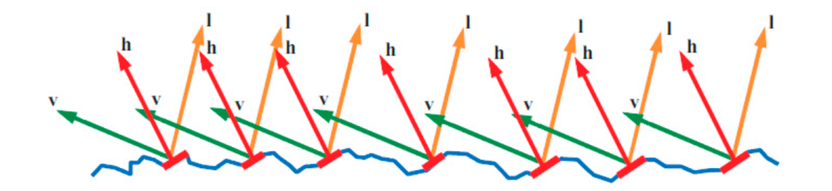
Microfacet 理论中存在以下三种事件：（a）表现 Masking，即出射光被微面遮挡，（b）表现 Shadowing，即入射光被微面遮挡，与（c）内反射，光路在微面内反射多次后来到视角。（图源 9.6 Roughness Using Microfacet Theory - “Three Important Geometric Effects to Consider with Microfacet Reflection Models”）

从宏观角度建模微观事件的手段往往是统计学——PBRT中使用 Trowbridge-Reitz （GGX） 分布来建模微面（Microfacet）理论。其中定义以下函数：

$D(w)$ - Microfacet Distribution，代表宏观平面上一点从视角$w$观察，「指向视角$w$」的微面比例；直觉的，以下式子，也即从所有视角观察到的面积分，成立： $$ \int_{H^2}{D(w_m)(w_m \cdot \mathbf n)dw_m} = 1 $$
$G(w)$ - Masking Function，代表宏观平面上一点从视角$w$观察，可被「直接观察到」的微面比例；类比平面情况（如图），我们也可以找到球面上他的积分的含义：从一定视角，所能“看到”的面的比例
在光滑平面下这是熟悉的$cos\theta = N\cdot L$；微面情景中，以下式子也应成立： $$ \int_{H^2}{D(w_m)G(w,w_m)(w_m \cdot \mathbf n)dw_m} = w \cdot \mathbf{n} = \cos\theta $$

两个重要的等式关系也将在后面推导VNDF采样中继续使用。GGX $D$, $G$本身的推导在此省略。

值得注意的是（c）情况在这里并未讨论，这里留了一个伏笔——之后在Multiscatter GGX中会再次提及…

VNDF

采样/利用$D$直接表达分布确实可以，但是我们有更优的方法。

回顾刚刚给出的第二个式子（往上划第一个）：在$w$视角观察下看得到的微观面比例为$cos \theta$。整理成以下形式： $$ \int_{H^2} \frac{D(w_m)G(w,w_m)(w_m \cdot \mathbf n)}{\cos\theta}dw_m = 1 $$ 左边的式子的积分是1！看起来是不是有PDF的感觉？而且这里“可见性”的概念也被$G$表达，实在方便。不妨拆出来记为$D_w(w_m)$： $$ D_w(w_m) = \frac{D(w_m)G(w,w_m)(w_m \cdot \mathbf n)}{\cos\theta} $$ 而这个式子就是VNDF方法——Visibile Normal Distribution Function，或可见法线分布函数的所在：不必采样完整的$D$，从视角出发，有多少就采样多少。

重要性采样

PBRT 书中的方法来自 Sampling the GGX Distribution of Visible Normals, Heitz 2018：其实很直觉——在前面，我们已经很清楚怎么采样一个均匀的半球Lobe：圆面投影半球；不妨将GGX的Lobe也“变形”成半球的形状，做同样的事情。

GGX的Lobe是个椭圆体：形状由我们提供的$\alpha$“粗糙度”决定。对各向异性情形则是$\alpha_x, \alpha_y$两个值，而将这个形状变回”圆“则很简单：平面本地切空间内表示($\mathbf n = (0,0,1)$)下，仅需一个缩放变换： $$ A = \begin{bmatrix}a_x & 0 & 0 \newline 0 & a_y & 0 \newline 0 & 0 & 0\end{bmatrix} $$ 之后，用缩放后的$n$去采样，采样方法和之前几乎一致。但值得注意的是，不同于漫反射：这里的Lobe可能并不完全在正平面内：

“裁切”掉这个情况并非难事：限制高度到$[cos\theta, 1]$即可。之后通过构造正交基就能把采样的向量投影做$A$的逆变换，回到正确的Lobe方向中

最后，我们完整的GGX采样实现如下。这里的PDF正是我们之前提到的$D$。

// https://www.pbr-book.org/4ed/Reflection_Models/Roughness_Using_Microfacet_Theory
// Trowbridge-Reitz (GGX) distribution/shadow-masking functions
public struct TrowbridgeReitzDistribution {
    float alpha_x;
    float alpha_y;
    public __init(float alpha_x, float alpha_y) {
        this.alpha_x = alpha_x;
        this.alpha_y = alpha_y;
    }
    // https://www.pbr-book.org/4ed/Reflection_Models/Roughness_Using_Microfacet_Theory#eq:tr-d-function
    // Distribution/percentage of microfacet normals at surface local point oriented towards wm
    public float D(float3 wm) {
        float tan2Theta = Tan2Theta(wm);
        if (isinf(tan2Theta)) return 0;
        float cos4Theta = Sqr(Cos2Theta(wm));
        float e = tan2Theta * (Sqr(CosPhi(wm) / alpha_x) +
                               Sqr(SinPhi(wm) / alpha_y));
        return 1 / (Pi * alpha_x * alpha_y * cos4Theta * Sqr(1 + e));
    }
    // Fallback to perfectly smooth case where PDF is dirac delta when true
    public bool EffectivelySmooth() {
        return max(alpha_x, alpha_y) < 1e-3f;
    }
    // Lambda for G1 masking-shadowing function at incident direction w
    public float Lambda(float3 w) {
        float tan2Theta = Tan2Theta(w);
        if (isinf(tan2Theta)) return 0;
        float alpha2 = Sqr(CosPhi(w) * alpha_x) + Sqr(SinPhi(w) * alpha_y);
        return (sqrt(1 + alpha2 * tan2Theta) - 1) / 2;
    }
    // Masking function for single incident direction
    public float G1(float3 w) { return 1 / (1 + Lambda(w)); }
    // Height-correlated Masking-Shadowing function (Smith G)
    // ---
    // * G1(wo)G1(wi) assumes independence - which is conservative and can lead to energy loss/darkening
    // * This correlates height fields - assumed as a NDF - to reduce energy loss
    public float G(float3 wo, float3 wi) {
        return 1 / (1 + Lambda(wo) + Lambda(wi));
    }
    // Normalized Visible Normal Distribution/VNDF
    // ---
    // For visible microfacets viewed from wm:
    //   \int_H^2 G1(w)G1(wm) max(0,w \cdot wm) dwm = w \cdot n = CosTheta(w) should hold
    // Thus we can derive the PDF for sampling visible normals with respect to incident direction w:
    //   D_w(wm) = \frac{G1(w)}{CosTheta(wm)} D(wm) max(0,w \cdot wm)
    public float D(float3 w, float3 wm) {
        return G1(w) / AbsCosTheta(w) * D(wm) * AbsDot(w, wm);
    }
    // Alias of D, the PDF for visible normal's importance sampling described below.
    public float PDF(float3 w, float3 wm) { return D(w, wm); }
    // Importance sampling of Visible Normals
    // ---
    // https://www.pbr-book.org/4ed/Reflection_Models/Roughness_Using_Microfacet_Theory#SamplingtheDistributionofVisibleNormals
    // See also "Sampling the GGX Distribution of Visible Normals" by Eric Heitz (https://jcgt.org/published/0007/04/01/paper.pdf)
    public float3 Sample_wm(float3 w, float2 u) {
        // 1. For anisotropic cases, transform the incident w back to a hemispherical configuration
        //    so we'd always work with a isotropic case.
        float3 wh = normalize(float3(alpha_x * w.x, alpha_y * w.y, w.z));
        if (wh.z < 0) wh = -wh; // Ensure wh is in the upper hemisphere
        // 2. Find a orthonormal basis around wh. This is PBRT's routine, though
        //    buildOrthonormalBasis [Frisvad, 2012] could be also used w/o normalization.
        float3 T1 = wh.z < 0.99999f ? normalize(cross(float3(0,0,1), wh)) : float3(1,0,0);
        float3 T2 = cross(wh, T1);
        // 3. Sample uniformly distributed point on a unit disk and project to clipped hemisphere
        float2 p = SampleUniformDiskPolar(u);
        float h = sqrt(1 - Sqr(p.x)); // Max height on hemisphere
        float s = (1 + wh.z) / 2;
        p.y = (1-s) * h + s * p.y; // Project to clipped hemisphere
        float pz = sqrt(max(0, 1 - LengthSquared(p)));
        float3 nh = p.x * T1 + p.y * T2 + pz * wh; // Apply TBN
        // 4. Reverse the anisotropic scaling to get the sampled microfacet normal
        return normalize(float3(alpha_x * nh.x, alpha_y * nh.y, max(1e-6f, nh.z)));
    }
}

注意几个细节：

PBRT提供了 EffectivelySmooth 方法，引导实现用前文介绍的镜面反射情况处理以避免（一定会出现且严重的）浮点数精度问题
这里的$G$函数同时表达Shadowing-Masking。在很多实现（如英伟达 https://github.com/nvpro-samples/nvpro_core2）及RTR4介绍中，混合Shadowing和Masking往往写成： $$ G_1(w_i)G_1(w_o) $$ 这蕴含着入射（shadowing）和出射（masking）事件不相关。PBRT指出这是过于保守的（太低），但相关性存在：试想一个很高的‘山峰’：从入射/出射两个角度都看不到。最后的形式来自 Understanding the Masking-Shadowing Function in Microfacet-Based BRDFs, Heitz 2014:
其中$\Lambda$已在实现中给出。

光泽反射（Torrance-Sparrow）

PBRT在介绍完漫反射后给出了ConductorBxDF及DieletricBxDF的定义——这里暂时不对他们进行直接介绍，但是其表达“粗糙度”的BRDF模型基础是一样的：来自 Theory for Off-Specular Reflection From Roughened Surfaces - Torrance, Sparrow 1967

之前提过对完全镜面/Specular情况的特殊处理，我们先很快地给出他PDF的定义：恒为0（回忆他是狄拉克函数$\delta(wi-wr)$）。对应的，其BSDF Eval（f）也为0,理解成球面上只「无穷小」的一点能表现入射光的「所有」能量：很显然，要表达将又是个无穷大，而这是做不到的。

雅可比行列式

图源RTR4 p337——建模微面BRDF时，利用half-vector （图中 $\mathbf h$，后面记为$w_m$）建模微面的法线会很方便，这点之后也能见识到。

不过去采样$w_m$有个问题：我们最后给「要的」是$w_i$。采样前者的话，二者并不在同一个空间内（绿色vs紫色）：

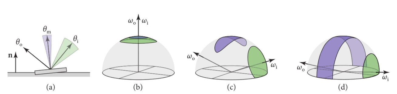
图源 PBRT。在（a）的平面情况，我们有简单的 $\theta_m = \frac{\theta_o + \theta_i}{2} $映射，他的雅可比行列式即$\frac{d\theta_m}{d\theta_i}=\frac{1}{2}$；而在(b),(c),(d)的球面中，立体角映射本身并不好找，但是他的雅可比行列式： $$ \frac{dw_m}{dw_i} = \frac{sin \theta_m d\theta_m d\phi_m}{sin \theta_i d\theta_i d\phi_i} $$ 是显然的。而球面中：

$w_i$是反射向量，那么$w_o,w_m$夹角等于$w_i,w_m$夹角，即有$\theta_i = 2\theta_m$；因此也有 $cos \theta_m = w_i \cdot w_m = w_o \cdot w_m$ 。这里和（a）也可以感受到
$w_o,w_m,w_i$共面，既有$\phi_m = \phi_i$

代入简化： $$ \frac{dw_m}{dw_i} = \frac{sin \theta_m d\theta_m}{sin 2\theta_m d2\theta_m} \newline \frac{dw_m}{dw_i} = \frac{sin \theta_m}{2sin 2\theta_m} \newline $$ 倍角公式： $$ \frac{dw_m}{dw_i} = \frac{sin \theta_m }{4sin \theta_m cos \theta_m} = \frac{1}{4 cos \theta_m} = \frac{1}{4 w_i \cdot w_m} = \frac{1}{4 w_o \cdot w_m} \newline $$

我们得到了这个变换的雅可比！接下来用于PDF计算也将马上用到。

f/Eval

和之前的VNDF理论一致，我们的分布也只关心“可见”部分。他的分布已经给出，但是$D_w(w_m)$是在half-vector空间的：好在我们已经知道了他到入射角变换的雅可比！

PDF $p_{(w_i)}$即为： $$ p_{w_i} = D_w(w_m) \frac{dw_m}{dw_i} = \frac{D_{wo}(w_m)}{4(w_o\cdot w_m)} $$

他的BRDF本身也很简单。同样回到渲染公式——引入单个样本蒙特卡洛的形式 $$ L_{\mathrm{o}}(\mathrm{p}, \omega_{\mathrm{o}}) = \int_{\mathrm{H}^2(\mathbf{n})} f_{\mathrm{r}}(\mathrm{p}, \omega_{\mathrm{o}}, \omega_{\mathrm{i}}) L_{\mathrm{i}}(\mathrm{p}, \omega_{\mathrm{i}}) |\cos \theta_{\mathrm{i}}| , \mathrm{d}\omega_{\mathrm{i}} \approx \frac{f_{\mathrm{r}}(\mathrm{p}, \omega_{\mathrm{o}}, \omega_{\mathrm{i}}) L_{\mathrm{i}}(\mathrm{p}, \omega_{\mathrm{i}}) |\cos \theta_{\mathrm{i}}|}{p(\omega_{\mathrm{i}})} $$

$w_o,w_i$已知的情况下是有解的：回顾之前$\cos\theta$和$G$的关系和菲涅耳公式表达的“反射率”，书中给出了这样的恒等关系： $$ \frac{f_{\mathrm{r}}\left(\mathrm{p}, \omega_{\mathrm{o}}, \omega_{\mathrm{i}}\right) L_{\mathrm{i}}\left(\mathrm{p}, \omega_{\mathrm{i}}\right)\left|\cos \theta_{\mathrm{i}}\right|}{p\left(\omega_{\mathrm{i}}\right)} \stackrel{!}{=} F\left(\omega_{\mathrm{o}} \cdot \omega_{\mathrm{m}}\right) G_{1}\left(\omega_{\mathrm{i}}\right) L_{\mathrm{i}}\left(\mathrm{p}, \omega_{\mathrm{i}}\right) $$ $p(w_i)$代入则有： $$ f_{\mathrm{r}}\left(\mathrm{p}, \omega_{\mathrm{o}}, \omega_{\mathrm{i}}\right) = p(w_i) \newline F\left(\omega_{\mathrm{o}} \cdot \omega_{\mathrm{m}}\right) G_{1}\left(\omega_{\mathrm{i}}\right) = \frac{D_{wo}(w_m) F(w_o\cdot w_m)G_1(w_i)}{4(w_o\cdot w_m)} $$ 代入VNDF： $$ f_{\mathrm{r}}\left(\mathrm{p}, \omega_{\mathrm{o}}, \omega_{\mathrm{i}}\right) = \frac{D(w_m) F(w_o\cdot w_m)G_1(w_i)G_1(w_o)}{4cos\theta_i cos \theta_o} $$ 回顾之前“细节”部分提到个高度相关$G(wi,wo)$，这里用上有： $$ f_{\mathrm{r}}\left(\mathrm{p}, \omega_{\mathrm{o}}, \omega_{\mathrm{i}}\right) = \frac{D(w_m) F(w_o\cdot w_m)G(w_i, w_o)}{4cos\theta_i cos \theta_o} $$ 此即Torrance-Sparrow BRDF的现代形式。

Sample_f/Sample

VNDF重要性采样和BRDF本身已经介绍过，这里用起来即可。代码将在之后实现各类BxDF时给出。

反射与折射

我们已经有了足够的数学工具建模光的「反射」概率模型。PBRT中，9.3 Specular Reflection and Transmission 被放在之前介绍，不过前面其实也只有一笔带过的菲涅耳$F$等很少的一部分需要这里的知识，索性拖到现在记笔记。

反射定律

现实中不存在完美的镜面：「能量」在接触表面后多少会被吸收：至于“多少”，这里之后同折射部分一并介绍。

不过就建模光路而言，满足入射角=出射角的情况一概归类于此：这里已在前面BxDF部分介绍过，不再多提。

折射定律

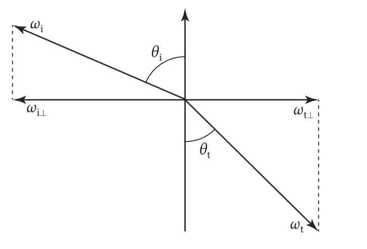
初高中学过的光的折射：斯涅尔定律（Snell’s Law） 告诉我们，光的折射角和入射角有以下关系（即入射面1,出射面2）

$$ \frac {\sin \theta_i}{\sin \theta_t} = n_{1,2}= \frac {n_1}{n_2}=\frac {v_2}{v_1} $$

其中折射率(Index Of Refraction, IOR) 记为 $n = \frac{n_t}{n_i}$ 。向量计算参考以下PBRT实现：

// https://www.pbr-book.org/4ed/Reflection_Models/Specular_Reflection_and_Transmission#SnellrsquosLaw
public bool Refract(float3 wi, float3 n, float eta /* IOR */, out float3 wt, out float etap){
    float cosTheta_i = dot(n, wi);
    if (cosTheta_i < 0) { // Inside an object?
        eta = 1 / eta;
        cosTheta_i = -cosTheta_i;
        n = -n;
    }
    float sin2Theta_i = 1 - Sqr(cosTheta_i);
    float sin2Theta_t = sin2Theta_i / Sqr(eta);
    if (sin2Theta_t >= 1) // Total internal reflection - transmission impossible
        return false;
    float cosTheta_t = SafeSqrt(1 - sin2Theta_t);
    wt = eta * -wi + (eta * cosTheta_i - cosTheta_t) * n;
    etap = eta;
    return true;
}

几个细节：

全反射情况下返回false，即光密到光疏的入射角$\theta_i > \theta_c = \sin^{-1}{\frac{1}{n}}$
etap接受假设介面为入射面时对应的折射率。计算即$\frac{1}{n}$

菲涅耳方程

实数折射率

之前提到的 $F_r$ - 菲涅耳定律给出了在光到材质上后，反射与折射「能量」的关系。计算本身涉及电磁相关波知识…大物好久没看也基本忘了，这里只给出形式

垂直(s)偏振的反射比为：

$$ R_{s}=\left({\frac {n_1\cos \theta_i-n_2\cos \theta_t}{n_1\cos \theta _i+n_2\cos \theta_t}}\right)^{2} $$

平行(p)偏振的反射比为： $$ R_{p}=\left({\frac {n_1\cos \theta_t+n_2\cos \theta_i}{n_1\cos \theta _t+n_2\cos \theta_i}}\right)^{2} $$
s,p偏振等量（无偏振）时，入射光的反射比即为：

$$ F_r={\frac {R_{s}+R_{p}}{2}}
$$

折射比很直接 $$ F_t = 1 - F_r $$

$\theta_i$已知，$\theta_t$的计算利用折射定律。以下即实数折射率计算反射比的PBRT实现：

// https://www.pbr-book.org/4ed/Reflection_Models/Specular_Reflection_and_Transmission#TheFresnelEquations
// Percentage of light reflected (or otherwise transmitted) at a dielectric interface
// with respect of incident angle theta and IOR eta
public float FrDielectric(float cosTheta_i, float eta) {
    // vv Same snippet for calculating Snell's law
    if (cosTheta_i < 0) { // Inside an object?
        eta = 1 / eta;
        cosTheta_i = -cosTheta_i;
    }
    float sin2Theta_i = 1 - Sqr(cosTheta_i);
    float sin2Theta_t = sin2Theta_i / Sqr(eta);
    if (sin2Theta_t >= 1) // Total internal reflection
        return 1.0f; // All scattering is in the reflection, no transmission component
    float cosTheta_t = SafeSqrt(1 - sin2Theta_t);
    // ^^
    float r_parl = (eta * cosTheta_i - cosTheta_t) /
                   (eta * cosTheta_i + cosTheta_t);
    float r_perp = (cosTheta_i - eta * cosTheta_t) /
                   (cosTheta_i + eta * cosTheta_t);
   return (Sqr(r_parl) + Sqr(r_perp)) / 2; // Power of both polarizations
}

在电介质材料里，该式子足矣建模其反射/折射能量关系——但对于导体而言则不是如此。

复数折射率

9.3.6 The Fresnel Equations for Conductors 介绍了折射率为$n - ik$的复数形式时的计算。实现如下：

// https://www.pbr-book.org/4ed/Reflection_Models/Specular_Reflection_and_Transmission#TheFresnelEquationsforConductors
// eta takes a complex form (IOR, k), where k is the absorption coefficient
public float FrComplex(float cosTheta_i, complex eta){
    cosTheta_i = clamp(cosTheta_i, 0, 1);
    // ^^ Ignore the case of inside an object for conductors as it's attenuated rapidly
    float sin2Theta_i = 1 - Sqr(cosTheta_i);
    complex sin2Theta_t = complex(sin2Theta_i) / Sqr(eta);
    complex cosTheta_t = sqrt(complex(1) - sin2Theta_t);
    complex r_parl = (eta * complex(cosTheta_i) - cosTheta_t) /
                     (eta * complex(cosTheta_i) + cosTheta_t);
    complex r_perp = (complex(cosTheta_i) - eta * cosTheta_t) /
                     (complex(cosTheta_i) + eta * cosTheta_t);
    return (norm(r_parl) + norm(r_perp)) / 2; // Power of both polarizations
}

$k$部分为「消光系数」，再次是一个测量值——金属的消光系数很大，以至于会对反射率产生不可忽略的影响：吸收（折射）多到光线无法穿透而变得不透明！

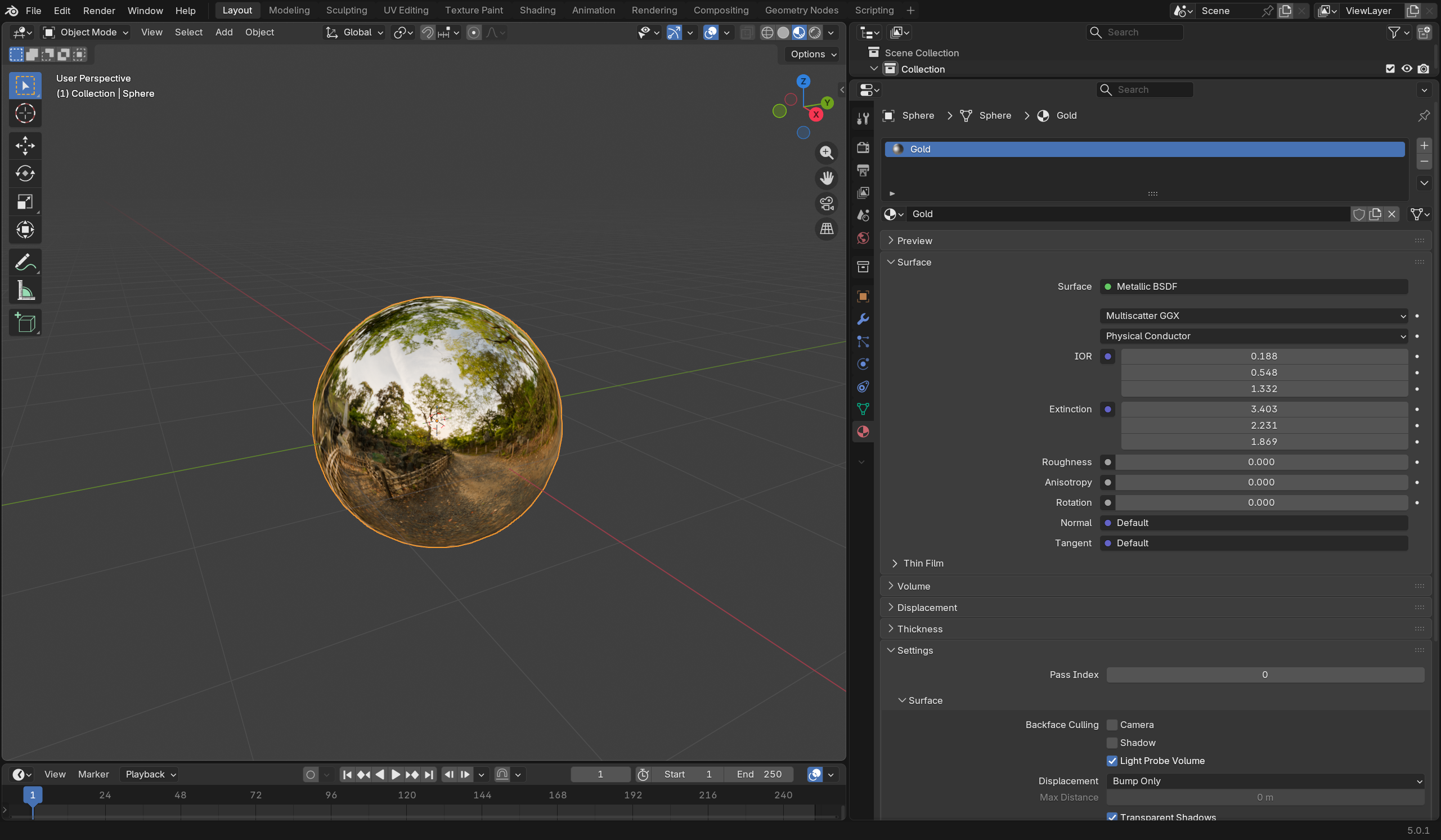
离线管线，和部分参考渲染器在建模金属时一般用的也是该形式：Blender也是如此。作为例子：

这个值和IOR一样，这个值和入射波长也有关系。RGB光谱$\lambda = (630nm,532nm,465nm)$下在 https://refractiveindex.info/?shelf=main&page=Rakic查表：

金子有$n=(0.18836,0.54836,1.3319), k=(3.4034,2.2309,1.8693)$ —— 插入 Blender 的 Metallic BSDF 中如下：

铝则为$n=(1.4303,0.93878,0.68603), k=(7.5081,6.4195,5.6351)$，如下：

n,k 估计

输入这两个测量值很麻烦。Artist Friendly Metallic Fresnel, Gulbrandsen 2014 给出了由两个RGB参数估计$n,k$的方法。这里只给出实现，来自 Blender Cycles：

// Approx F0 to Complex Fresnel IOR terms
// "Artist Friendly Metallic Fresnel", Gulbrandsen 2014, https://jcgt.org/published/0003/04/03/paper.pdf
public void FresnelFromF0(float r /* baseColor */, float g /* specularTint */, out float n, out float k){
    r = clamp(0.01, 0.99, r);
    float sqrt_r = sqrt(r);
    n = lerp((1.0f + sqrt_r) / (1.0f - sqrt_r), (1.0f - r) / (1.0f + r), g);
    k = SafeSqrt((r * Sqr(n + 1) - Sqr(n - 1)) / (1.0f - r));
}
public void FresnelFromF0(float3 r /* baseColor */, float3 g /* specularTint */, out float3 n, out float3 k){
    for (int i = 0; i < 3; i++)
        FresnelFromF0(r[i], g[i], n[i], k[i]);
}

以上即为对电介质和导体反射率计算所需的一切工具。他们在接下来的材质建模会变得很方便！

PBRT里介绍的 9.4 Conductor BRDF, 9.5 Dielectric BSDF暂不直接记录：他们将间接地在接下来的模型中得到体现。

glTF 材质模型

毕竟到目前为止，glTF是我们唯一的场景格式。要实现则需要把他的材质模型映射到我们目前PBRT风格的BxDF中。

pbr

上图来自 glTF 2.0 Spec Appendix B——glTF在电介质和导体间做线性插值，做法对应PBRT的 MixMaterial。对两者材质本身而言：

电介质模型

glTF的该模型可以认为是和PBRT中的DieletricBxDF与DiffuseBxDF做的LayeredBxDF的“简化”版本：上层光泽层「反射]+「折射」到下层漫「反射」再次「折射」出介面。

不过，注意图中x部分：这里的层次间叠加(fresnel_mix)不考虑介面间的反射，二次反射会直接被忽略，能量消失！

再次地，这是一个single-scattering模型：所谓“简化”就是这个意思。PBRT中在介面多次NEE做Random Walk，还需考虑介面厚度及衰减问题…这是ground truth答案，虽然跑起来会很慢。在此，我们只做一次 NEE——这不可避免地会产生能量损失，但这个问题可以留给未来的自己解决…

导体模型

不必担心，这里（假设metallic=1）的表现和ConductorBxDF是一致的。我们已经介绍过他的（复数）$F_r$，插入之前我们的光泽反射BSDF即可得到导体情况的BSDF。

fresnel_mix 的由来

可以看到，电介质材质有两个BRDF Lobe需要采样：光泽$w$和漫反射$w\prime$。BRDF间的混合并非加法：这样做很显然是能量不守恒的。但从采样的角度出发：在一个点上，这两个$w$都可能是被采样到的光线（参考上图）。如果知道这两者采样**「可能性」**的话，岂不是可以做任意选择而去逼近混合后的结果？

这既是LayeredBxDF中用到的NEE/Next Event Estimation（次事件估计）的思想。而回顾我们之间讨论过的菲涅耳方程：我们很清楚有**「多少」**能量会到达下一层（然后反射），又有多少会被直接反射：_反射率_表达了这样的比例！

当然，这里的比例并不精确——实际上这再次地是一个single scattering模型：ground truth则是PBRT中介面的混合是用 Random Walk 来做的 LayeredBxDF。这方面的补偿会在后面讨论。

菲涅耳项估计

计算菲涅耳本身在之前介绍过——而前面用了ShlickFresnel。当然，mix FrDieletric和FrConductor在这里是正确的…但用到的三角函数是不是有些多？

此外，glTF对导体BSDF的表达依赖于RGB BaseColor。我们确实也知道如何估计表现他的$n,k$折射率及消光系数（见前文）——但在此有无必要则值得思考。

在各种glTF光栅器及实时渲染工具中，用到的并非之前从波向量出发的计算方式，而是以下估计形式，来自An Inexpensive BRDF Model for Physically-based Rendering, Shlick 1994 $$ {\displaystyle R(\theta )=R_{0}+(1-R_{0})(1-\cos \theta )^{5}} \newline {\displaystyle R_{0}=\left({\frac {n_{1}-n_{2}}{n_{1}+n_{2}}}\right)^{2}} $$ 用$n=\frac{n1}{n2}$表示 $$ R_0 = (\frac{n-1}{n+1})^2 $$

实现很简洁，如下：

public float SchlickFresnel(float F0, float F90, float cosTheta)
{
  return F0 + (F90 - F0) * pow(1.0F - cosTheta, 5.0F);
}

能量守恒改进

暂时不贴代码：进行白炉测试，可以发现：粗糙度越高球体变得越暗。同时，球体边缘部分情况更严重。

后者来自我们之前讨论过的到漫反射面的单次折射——这是非常保守的，以至于粗糙度变高时，无法一次折射大部分的光线会消失，边缘变暗。

此外，还记得之前讨论微面情况（c）的内反射：GGX是不处理，而当作被“吸收”而显得更“暗”。真实材质确实可能吸收能量，但对我们目前的建模而言这不应该。这里在glTF Spec中也有提及：

Microfacet models often do not consider multiple scattering. The shadowing term suppresses light that intersects the microsurface a second time. Heitz et al. (2016) extended the Smith-based microfacet models to include a multiple scattering component, which significantly improves accuracy of predictions of the model. We suggest to incorporate multiple scattering whenever possible, either by making use of the unbiased stochastic evaluation introduced by Heitz, or one of the approximations presented later, for example by Kulla and Conty (2017) or Turquin (2019).

接下来就Heitz方法简要介绍，并对这里的Kulla and Conty方法进行复现。

Random Walk (Heitz 2016)

记得$G1$ Masking/Shadowing 函数表达的量：宏观面内沿某视角$\mathbf{v}$可见的微面比例。

而现在所用的Single Scattering模型会导致折射接触到的面贡献被忽略，但现实中是能继续反弹出来的：图源 4.7.2 Energy loss in specular reflectance。Roughness越大，散射走的越多，能量损失越大，这可以解释“变暗”情况。

在微面内完整光路的ground truth方法由 Multiple-Scattering Microfacet BSDFs with the Smith Model, Heitz 2016 提出，在 Blender 4.0 之前 (3.6.x) 也是其Multiscatter GGX的实现。

概述如下：设微面高度分布为NDF/正态分布，从初始方向多次“walk”这些“峰”，并相应地反射，重复执行到轮盘赌或迭代上限达到位置。

计算量…非常大。Random Walk方法在之前的LayeredBxDF中也见到过，我们因此也暂时没有用它。

未来有机会再尝试复现这里的RW手段。在此之前，实现上更为简单且出图方差更低（不需逼近）的手段即为以下查表方法。

预积分查表（Kulla, Conty & Turquin）

Blender 4.0 以后采用了查表方法(注意cycles做的$E_{avg}$等查表）。形式上是后者Turquin的公式，不过鉴于其推导离不开Kulla 2017的工作，这里一并复现。方便读者参考，以下为二者链接：

方向反照率 Albedo $E(w)$

设想：白炉中的有一球体，他的BRDF为$\rho(w_o,w_i)$，$F = 1$：以下积分是一定成立的，即上图的式子（d）（来自 Understanding the masking-shadowing function in microfacet-based BRDFs - Heitz 2014 ) $$ E(w_o) = \int_{H^2}{\rho(w_o,w_i) cos\theta d\omega} = 1 $$ 以上则为反照率/Albedo的定义，朝任意方向，对反射率为1的物体，在白炉中应有反照率$Albedo=1$。

但我们已经知道包括GGX在内的微面模型并不包含内反射（前文情况c）能量，定义上则存在能量损失；Heitz在这篇论文中指出可以从如何「补偿」这部分丢失的能量出发；设单次散射模型为$\rho_{ss}(w_o,w_i)$,补偿量为$\rho_{ms}(w_o,w_i)$，应有： $$ \rho(w_o,w_i) = \rho_{ss}(w_o,w_i) + \rho_{ms}(w_o,w_i) $$

设同样的积分，代入前面能量守恒关系有： $$ E(w_o) = E_{ss}(w_o) + E_{ms}(w_o) = 1 \newline E_{ms}(w_o) = 1 -E_{ss}(w_o) $$

为方便后面计算，我们用$\mu=\cos\theta$表示入射角（假设$\phi$无关——在Kulla-Conty方法中如此），可以得到： $$ E(\mu_0) = \int_{0}^{2\pi}{\int_{0}^{1}}f(\mu_0, \mu_i)\mu_id\mu_id\phi \newline E(\mu_0) = 2\pi\int_{0}^{1}f(\mu_0, \mu_i)\mu_id\mu_i \newline $$ 作为验证，我们可以代入漫反射的BRDF $f_r = R/\pi$, 并令$R=1$： $$ E(\mu_0) = 2\int_{0}^{1}\mu_id\mu_i = 1 $$

平均反射率 $F_{avg}$

假设能量确实守恒的话，从一点，假设环境光照均匀——平均能反射出多少光？平均反射率表述的就是这一点：在没有任何遮蔽的情况下（包括shadowing-masking），上半球余弦加权的反射率积分。其能量形式如下： $$ \int_{H^2} F(\theta) cos\theta d\omega $$ 立体角拆开来： $$ \int_{0}^{2\pi}{\int_{0}^{\frac{\pi}{2}}}{F(\theta)cos\theta sin\theta d\theta d\phi} $$ $\phi$无关，提出$2\pi$ $$ 2\pi \int_{0}^{\frac{\pi}{2}}{F(\theta)cos\theta sin\theta d\theta} $$ 换元积分$u = cos\theta$ $$ 2\pi \int_{0}^{1}{F(\theta)u du} $$ 这是平均反射的「能量」。我们假设的“均匀环境光下”的入射能量很简单——还记得CosineHemispherePDF是怎么推导出来的： $$ i = \int_{H^2}{cos\theta}d\omega = \pi $$ 他们的比例则是得到平均反射率值，即为： $$ 2 \int_{0}^{1}{F(\theta)u du} $$ $F(\theta)$的原形式积分很麻烦。这里 Blender 用了之前介绍的 Shlick 估计，代入有 $$ 2 \int_{0}^{1}{ (R_{0}+(R_{90}-R_{0})(1-u )^{5}) u du} $$ 常数拆掉，不妨指数设为$n$，这里即为Blender Cycles中的形式。$s$对于一定的$n$是个常数

附注：此为 4.7.2 Energy loss in specular reflectance “魔法数字”的来源：对$n=5(Shlick)，s=2/(42)=1/21$

$$ s = 2 \int_{0}^{1}{ (1-u)^{n} u du} = \frac{2}{(n+3)n + 2} $$

常数补回来如下： $$ F_{avg} = R_0 + s(R_{90} - R_0) = lerp(R_0, R_{90}, s) $$

平均反照率 $E_{avg}$

在同样环境下,方便起见，我们对$E_{ss}$求一个相似概念：平均反照率（Average Albedo） $$ E = \int_{H^2}{E_{ss}(\omega)cos\theta d\omega} $$ 在此$\phi$无关，简化: $$ E = 2\pi \int_{0}^{\frac{\pi}{2}}{E_{ss}(\theta)cos\theta sin\theta d\theta} $$ 再次换元$\mu=cos\theta$ $$ E = 2\pi \int_{0}^{1}{E_{ss}(\mu)\mu d\mu} $$ 入射能量再次是$\pi$ - 这里和之前一样。得到反照率为： $$ E_{avg} = 2\int_{0}^{1}{E_{ss}(\mu) \mu d\mu} $$ 式子和$F_{avg}$推导基本一致。这样我们也能算出平均丢失能量，即为$1-E_{avg}$

$E,E_{avg}$ 预积分

回顾前文，$E, E_{avg}$的计算都需要积分，而且（GGX）分析解找不到。参考Blender cycles_precompute.cpp - 接下来给出通过采样预计算这两个值的方法。和前文一致，$\phi$被视作无关。

$E$的蒙特卡洛形式为： $$ E(\mu_0) = \int_{0}^{2\pi}{d\phi}\int_{0}^{1}f(\mu_0, \mu_i)\mu_id\mu_i = \frac{1}{N}\sum \frac{f(\mu_o, \mu_i)\mu_i}{p(\mu_i)} $$

同样的，对于$E_{avg}$，直接代入上面$E$的单个样本形式： $$ E_{avg} = 2\int_{0}^{1}{\mu d\mu \times E(\mu) } = \frac{1}{N}\sum \frac{2\mu_o \times f(\mu_o, \mu_i)\mu_i}{p(\mu_i)} $$ 无视仰角$\phi$，我们的$\mu$到$\omega$为简单的半圆面关系： $$ \omega = (sin \theta,0,cos\theta) = (\sqrt{1-\mu^2},0,\mu) $$ 实现工作已准备就绪。以下为Slang部分代码：

// Reference: https://projects.blender.org/blender/blender/src/commit/00546eb2f34cc95976a640d268deb371b7ca9210/intern/cycles/app/cycles_precompute.cpp
import "../Editor/Shaders/IMath";
import "../Editor/Shaders/IBRDF";
RWStructuredBuffer<float> output : register(u0);

float sampleGGX_E(float rough, float cosTheta, float uc, float2 u){
    float alpha = Sqr(rough);
    TrowbridgeReitzDistribution mfDistrib = TrowbridgeReitzDistribution(alpha, alpha);
    if (mfDistrib.EffectivelySmooth())
        return 1.0f; // Dirac delta - though we're counting energy, so return 1
    float3 wo = float3(sqrt(1.0 - cosTheta * cosTheta), 0.0, cosTheta);
    float3 wm = mfDistrib.Sample_wm(wo, u);
    float3 wi = Reflect(wo, wm);    
    if (!SameHemisphere(wo, wi))
        return 0.0f; // Absorption
    float pdf = mfDistrib.PDF(wo, wm) / (4 * AbsDot(wo, wm));
    float f = mfDistrib.D(wm)  * mfDistrib.G(wo, wi) / (4 * AbsCosTheta(wi) * AbsCosTheta(wo));
    return f * AbsCosTheta(wi) / pdf;
}

[shader("compute")]
[numthreads(32,32,1)]
void integrateGGX_E(uint2 p : SV_DispatchThreadID)
{
    static const uint kSamples = 1 << 12;
    float sum = 0.0f, samples = 0.0f;
    float u = (float(p.x) + 0.5f) / 32.0f, v = (float(p.y) + 0.5f) / 32.0f;
    PCG rng = PCG(uint4(p, 0, 0));
    for (uint i = 0; i < kSamples;i++) {
        float cosTheta = clamp(u, 1e-4, 1.0f);
        float rough = clamp(v, 1e-4, 1.0f);  
        sum += 1 - sampleGGX_E(rough, cosTheta, rng.sample(), rng.sample2D());
        samples += 1.0f;        
    }
    output[dot(p, uint2(1, 32))] = sum / samples;
}

[shader("compute")]
[numthreads(32,1,1)]
void integrateGGX_Eavg(uint2 p : SV_DispatchThreadID)
{
    static const uint kSamples = 1 << 14;
    float sum = 0.0f, samples = 0.0f;
    float u = (float(p.x) + 0.5f) / 32.0f;
    PCG rng = PCG(uint4(p, 0, 0));
    for (uint i = 0; i < kSamples;i++) {        
        float cosTheta = rng.sample();
        float rough = clamp(u, 1e-4, 1.0f);  
        sum += 2 * cosTheta * sampleGGX_E(rough, cosTheta, rng.sample(), rng.sample2D());
        samples += 1.0f;        
    }
    output[dot(p, uint2(1, 32))] = sum / samples;
}

Slang 写 Kernel？

Foundation 现在还没有给这种one-shot运行出结果的CS搭脚手架。这当然很有用，不过这并非我们「渲染」引擎想去解决的问题。

我们用的Shader语言Slang为「科学计算」提供了不少奇技淫巧：支持自动微分，多架构CPU/GPU执行：而且是write once, run everywhere那种！

利用slangpy ——你甚至可以用Jupyter Notebook跑HLSL/GLSL做kernel，并且可选地带GPU加速！~~学术性游戏开发~~

不过要是有的选大家还是会用CUDA吧…

以下演示产生查表LUT的Notebook。Python利用slangpy代码部分非常简单，大致如下：

import slangpy
device = slangpy.create_device(slangpy.DeviceType.vulkan)
program = (cwd / "CSPrecompute.slang").as_posix()    

integrateGGX_E = device.create_compute_kernel(device.load_program(program, ["integrateGGX_E"]))    
integrateGGX_Eavg = device.create_compute_kernel(device.load_program(program, ["integrateGGX_Eavg"]))

ggx_E = device.create_buffer(element_count=32*32, struct_size=4, format=slangpy.Format.r32_float, usage=slangpy.BufferUsage.unordered_access)
ggx_Eavg = device.create_buffer(element_count=32, struct_size=4, format=slangpy.Format.r32_float, usage=slangpy.BufferUsage.unordered_access)

integrateGGX_E.dispatch(thread_count=[1,1,1],vars={"output": ggx_E})
integrateGGX_Eavg.dispatch(thread_count=[1,1,1],vars={"output": ggx_Eavg})

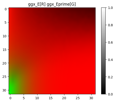
在Notebook中的输出如下。注意这里显示的并非$E$，而为$1-E$的积分：这是为了和Kulla的演示对比。

Kulla, Conty	复现

类似的，可以计算$E_{avg}$的值。见下图：$x$ 轴为$rough$，可见到最后能量的丢失高达60%!

幸运的是，这个值是值得相信的。在Practical multiple scattering compensation for microfacet models - Turquin 2019 中，作者对几个microfacet模型的能量损失提了一笔：的确，不考虑$F$项的GGX在此时确实会有如此之大的能量损失！

就此，我们给出的几个积分计算完毕。

$f_{ms}$ 推导

先不考虑反射率，Revisiting Physically Based Shading at Imageworks - Kulla, Conty 2017 给出了以下$f_{ms}$补偿BRDF中的Fresnel（ss:single scattering, ms: multiple scattering）：

$$ f_{ms}(w_o,w_i) = \frac{(1-E_{ss}(w_o))(1-E_{ss}(w_i))}{\pi(1-E_{avg})} \newline f\prime = f_{ss} + f_{ms} $$

这个式子由 A Microfacet Based Coupled Specular-Matte BRDF Model with Importance Sampling - Kelemen 2001 找到（下图）

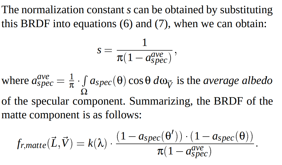
代入$E_{ms}$计算积分满足$E_{ss} + E_{ms} = 1$关系。如果$E_{avg}$已知的话，$f_{ms}$则能被轻易算出。我们之前已经完成了这部分的工作！

不过注意，目前为止的公式都做了一个简化假设：$F=1$——表现实际的反照率则需打破因此带来的$E(\mu)=1$ 假设。

幸运的时，目前为止我们算的都是「平均量」。$F\ne1$的「能量」损失也是易得的。回顾之前的反射率定义，「一次平均」反射返回的能量为： $$ F_{avg}E_{avg} $$ 继续：「之后」面介面内的反射呢？我们知道在（c）情况，不记$F$，内部反射丢失的平均能量是$1-E_{avg}$：结合之前的$F_{avg}$，则有次反射「丢失」的能量为 $$ l = F_{avg}(1-E_{avg}) \newline \Delta{E} = F_{avg}E_{avg}l $$ 然后，未丢失部分能量继续反射，反反复复…直到被完全吸收。那中途「丢失」的能量和，是不是有头绪计算了？

是的——这里有一个等比数列！丢失的能量总和即为： $$ \sum_{k=1}^{\infty}{\Delta{E}} = F_{avg}E_{avg}\sum_{k=1}^{\infty}{l^k} = F_{avg}E_{avg}\frac{l}{1 - l} = \frac{F^2_{avg}E_{avg}(1 - E_{avg})}{1 - F_{avg}(1 - E_{avg})} $$ 最后，$F_{avg}=1$时这个式子也恒等于$1 - E_{avg}$：这也是成立的。

反映到之前的$f_{ms}$，Kulla把这个和直接作比例乘回$f_{ms}$了——这是不对的（读者请思考$F_{avg}=1$时情况）。在原Talk Appendix中这也被修正：最后对应所有$F$的$f_{ms}$即为： $$ f_{ms}\prime =\frac{(1-E_{ss}(w_o))(1-E_{ss}(w_i))F^2_{avg}E_{avg}}{\pi(1-E_{avg})(1 - F_{avg}(1 - E_{avg}))} $$ 幸运的是，这正是 Filament 4.7.2 Energy loss in specular reflectance 用的式子！不过有点长，假如可以简化…

$f_{ms}$ 简化

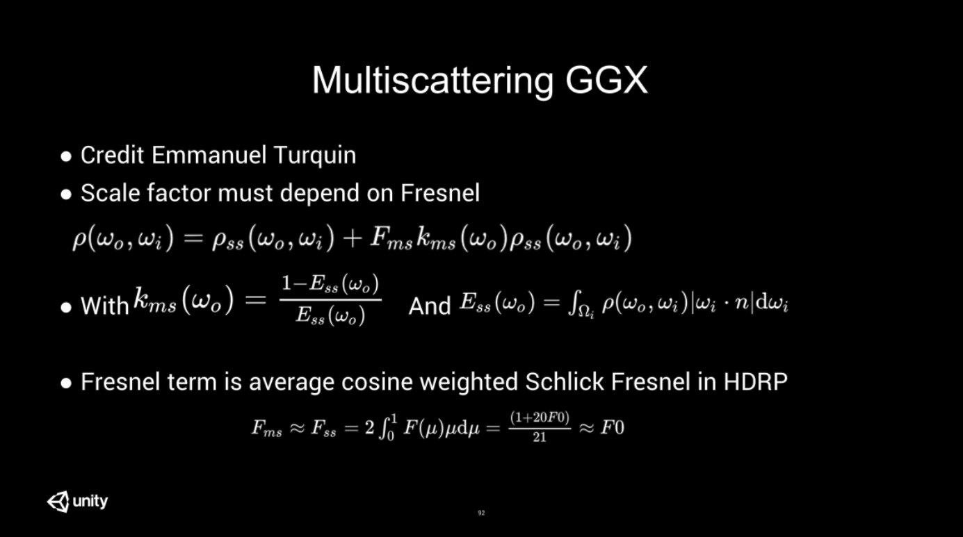
在 The road toward unified rendering with Unity’s high definition rendering pipeline, Lagrade 2018 中就有提及，Turquin在后来自己在2019的技术报告中也给出了一样的形式。

核心观察是：正如我们之前所见，$F_{avg}$是个很小的值(记得之前推导的Shlick 模型，$n=5, s= 1/21$)，$F_{ms}$不妨直接不算…

此外，另外的好处是，因为这样的计算相当于是对原Lobe进行“缩放”…

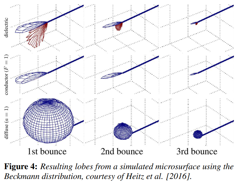
这和Heitz跑出来的实际情况是很像的：多次反射/multiscatter的lobe很像第一次单次折射的lobe！

之前没有提及，但是Kulla的方法（记得不记$\phi$）的补偿lobe是一个简单的diffuse/半球lobe；参考上图，可见Turquin的方法会更接近物理事实。

最后，非常简单的补偿量$f_{ms}$即为 $$ f_{ms} = f_0 \frac{1-E}{E}f_{ss} = f_0 (\frac{1}{E} - 1)f_{ss} $$

这里加到我们的glossy lobe即可。对glTFBSDF的Sample_f部分改进：

...
float mu = AbsCosTheta(wo);
float rough = sqrt(max(mfDistrib.alpha_x, mfDistrib.alpha_y));
float E = ggxLutE.SampleLevel(lutSampler, float2(mu, rough), 0);
float3 Fss = SchlickFresnel(F0, 1.0f, ClampedDot(wo, wm));
float3 Fms = F0 * (1/E - 1) * Fss;
float3 f = (Fss + Fms) * mfDistrib.D(wm) * mfDistrib.G(wo, wi) / (4 * AbsCosTheta(wi) * AbsCosTheta(wo));
return BSDFSample(f, wi, pdf, BxDFFlags::GlossyReflection);

导体

导体效果

一样的白炉测试效果如下。先令所有metallic=1.0f,即只看ConductorBxDF等效部分：

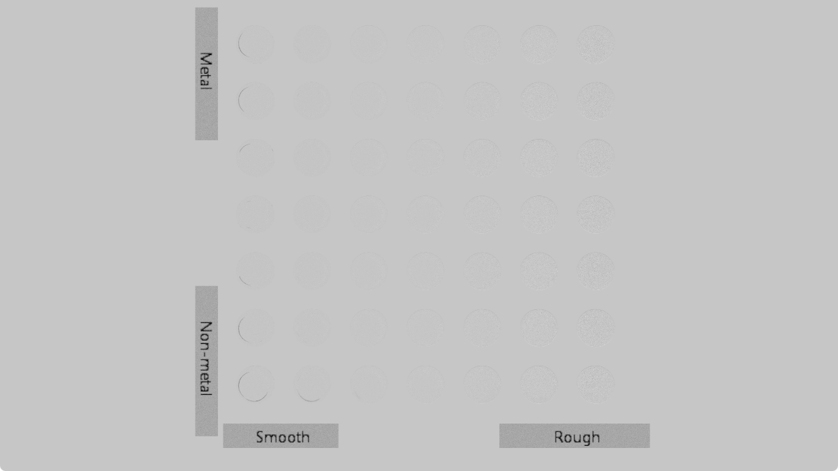
(注：别忘了Sampler用CLAMP_TO_EDGE - -||)

电介质

目前为止，我们只对不存在（不考虑：导体中折射即吸收）折射贡献的BRDF做了改进。对于电介质BRDF（及metal<1），这里的工作是不够的：因为算$E$的时候并没有看「折射」后的能量问题。

有一个问题就是这里的参数多了个IOR，ImageWorks (Kulla, Conty)提出使用3D材质查表。不过进行一些数学观察不难发现，这个表其实可以仅用两张表达所有$F_0, F_{90}$的情况。

电介质$E(\mu)$

回顾之前不考虑$F$（设$F=1$）的$E$计算，和其对应离散/蒙特卡洛形式： $$ E(\mu_0) = \int_{0}^{2\pi}{d\phi}\int_{0}^{1}f(\mu_0, \mu_i)\mu_id\mu_i = \frac{1}{N}\sum \frac{f(\mu_o, \mu_i)\mu_i}{p(\mu_i)} $$ 和之前一样，这里引入$F$即可；鉴于我们使用Shlick形式且IOR=1.5，则有： $$ F = f_0 + (f_{90} - f_{0}) \times (1.0 - \cos\theta)^5 $$

麻烦，多了个$f_0, f_{90}$；不妨拆成几个项，记： $$ \lambda(\theta) = (1.0-\cos\theta)^5 $$ 我们求的是： $$ E(\mu_0) = \int_{0}^{2\pi}{d\phi}\int_{0}^{1}F(w_o \cdot w_m)f(\mu_0, \mu_i)\mu_id\mu_i \newline $$

化简： $$ E(\mu_0) = f_0 \int_{0}^{2\pi}{d\phi}\int_{0}^{1}f(\mu_0, \mu_i)\mu_id\mu_i + (f_{90}-f_0) \int_{0}^{2\pi}{d\phi}\int_{0}^{1}\lambda(w_o \cdot w_m)f(\mu_0, \mu_i)\mu_id\mu_i $$ 常数$f_0,f_{90}$完全可以拖出来。此外，注意到左边积分还是之前$E$的形式；右边多了个$\lambda$，额外记一个表算即可。我们记右边（不包括$f_0,f_{90}$的积分为$E\prime$，离散形式为： $$ E\prime(\mu_0) = \int_{0}^{2\pi}\int_{0}^{1}\lambda(w_o \cdot w_m)f(\mu_0, \mu_i)\mu_id\mu_i = \frac{1}{N}\sum \frac{\lambda(w_o \cdot w_m)f(\mu_o, \mu_i)\mu_i}{p(\mu_i)} $$ 最后的$E\prime\prime(\mu_0)$则为: $$ E\prime\prime(\mu_0) = f_0 \times E(\mu_0) + (f_{90} - f_0)\times E\prime(\mu_0) $$ 和之前计算相比改动很小。直接贴代码：

// sampleGGX_E 额外输出 VdotH
float3 wo = float3(sqrt(1.0 - cosTheta * cosTheta), 0.0, cosTheta);
if (mfDistrib.EffectivelySmooth()){
    float3 wi = float3(-wo.x, -wo.y, wo.z);
    float3 wm = normalize(wo + wi);
    VdotH = AbsDot(wo, wm);
    return 1.0f; // Dirac delta - though we're counting energy, so return 1
}    
float3 wm = mfDistrib.Sample_wm(wo, u);
VdotH = AbsDot(wo, wm);
// integrateGGX_E 多一项 E'
for (uint i = 0; i < kSamples;i++) {
    float cosTheta = clamp(u, 1e-4, 1.0f);
    float rough = clamp(v, 1e-4, 1.0f);
    float3 wi;          
    float VdotH;
    float sample = sampleGGX_E(rough, cosTheta, rng.sample(), rng.sample2D(), VdotH);        
    float lambda = pow(1 - VdotH, 5);
    E += sample;
    Eprime += lambda * sample;
    samples += 1.0f;        
}
ggxE[dot(p, uint2(1, 32))] = float2(E / samples, Eprime / samples);

跑出来是这样的。参照不太好找，不过 Filament 5.3.4.3 The DFG1 and DFG2 term visualized 做了类似的事情：事实上我们的$E\prime$和$DFG_2$是一致的，对比如下（作为对比:R实际为(1-λ)*E, 同时这里的Y轴有翻转处理以对齐Filament结果）

Filament	Ours

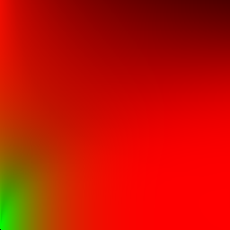实际载入使用的则为以下形式：UV顺序上和ImageWorks与自己之前的LUT一致。

电介质效果

ImageWorks也提到了对Diffuse lobe的调整（虽然这部分我们也讨论过了）：$E\prime\prime$是补偿过的反射量，那么真正能到达底层diffuse lobe的能量即为$1-E\prime\prime$（回顾反射率关系），刚好允许我们进行正确的能量调整：漫反射一定有入射=出射，$1-E\prime\prime$则是混合glossy lobe后其正确的反照率。

至此电介质模型调整完毕。让metallic=0（全电介质）的效果如下：

总结

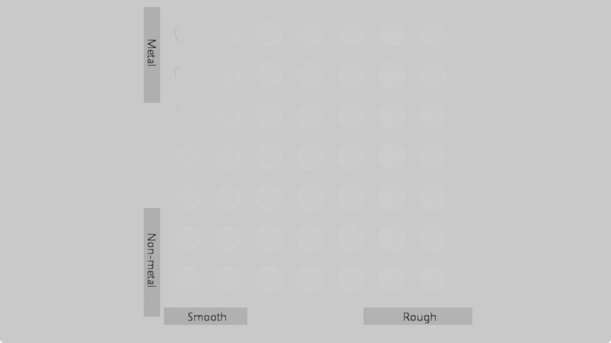
最后，调整完能量守恒前后的该模型在白炉测试中效果如下：

实现部分还有很多细节，尽力也在注释中标注。这里就不贴出来了——有兴趣还请看仓库链接：https://github.com/mos9527/Foundation/blob/vulkan/Editor/Shaders/IBSDF.slang （可能有死链…届时请在在仓库搜索 PrincipledBSDF 然后..留个言提醒下？）

样张

Tonemap部分和上一篇一致。灯光采样用到了 MIS（Multiple Importance Sampling, 虽然现在就只支持太阳光+环境光..），但PBRT灯光采样章节只是略过看了下。期末结束放假再来搞搞IBL和many light…

此外，自己的渲染器是没有降噪的；同时 glTF 不会存储曝光设置需要手动调整，同Cycles对比场景的亮度会有些许偏差。

最后放几张渲染器在几个样例场景中的表现。

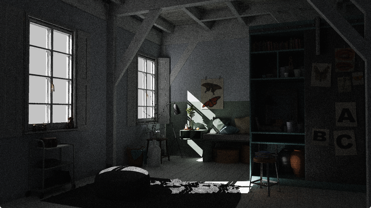
Evermotion - Archinteriors vol. 48 - 008

生产级场景（3M多边形），在Gems书上第十四章也出现过。光泽材质比较少，MIS做对后要达成相似输出还是比较容易的。

链接…无可奉告 ~~（蛤？）~~ 原因是Evermotion 还在卖这些场景。你问我买了没有：买了。~~不过是在淘宝买的百度云链接（~~

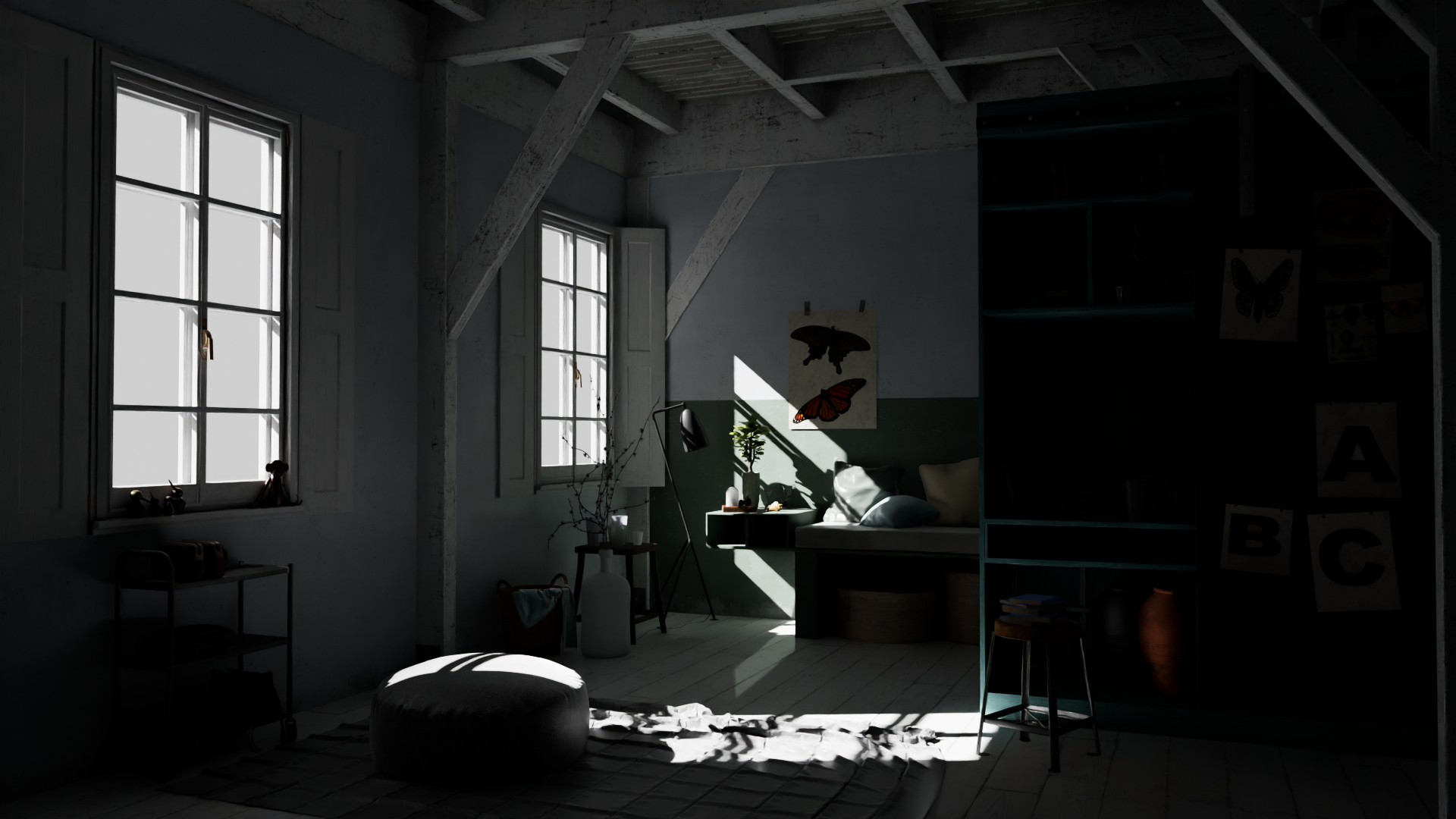
下面是Blender (5.0.1 LTS) Cycles在同样场景的渲染结果：开启降噪，Tonemapper为ACES1.3

Cycles 参考

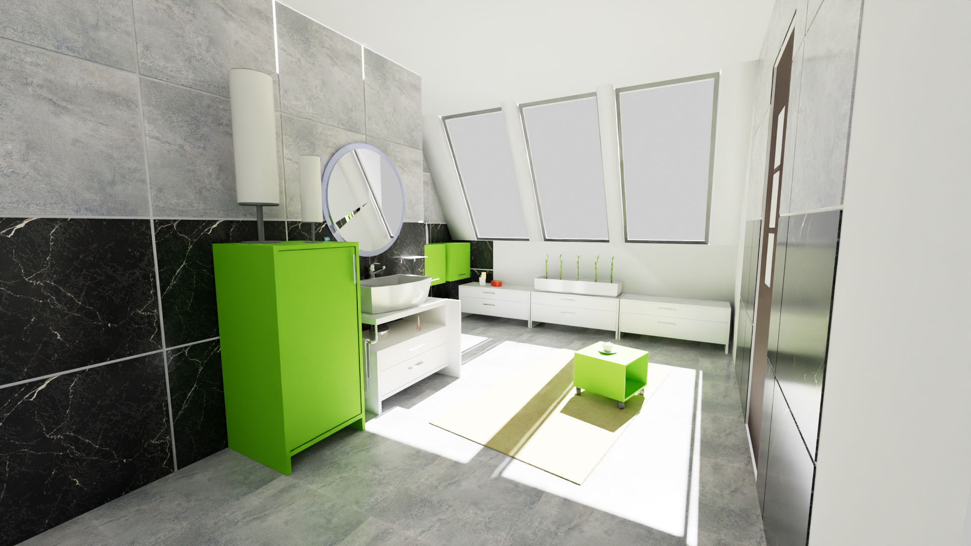
referencePT Bathroom

很英伟达的浴室，来自 Ray Tracing Gems 2 提到的 https://github.com/boksajak/referencePT/tree/master/models/bathroom

这次不少材质都是光泽的（同时包括完美镜面）；Blender的Prinicpled BSDF用Multiscatter GGX保持他们的能量守恒（之前介绍过）——注意洗手台和瓷砖的表现：这里很幸运地和Blender输出一致。

Cycles与之前一个设置的渲染结果如下：

Cycles 参考

Lumberyard Bistro

来自 https://github.com/zeux/niagara_bistro。植被渲染需要透明度支持，这里现存的naive实现too simple：他很慢 —— anyhit跑一遍，shadow ray还要跑一遍，没考虑mip就采样等等。

不过最近没啥时间继续折腾了。透明度方面的效率问题，仍然留给未来的自己解决…

Cycles 参考

Blender Classroom

来自 https://www.blender.org/download/demo-files/

原Blend用的BSDF有些魔幻（glossy手动mix diffuse，然后各种奇怪混合方式弄roughness map），算不上现代metal-rough PBR模型资产

结果就是基本手动调了一遍。此外因为没有volume rendering，原场景的体积光在此没有加入。

直接光源+多个自发光光源演示。

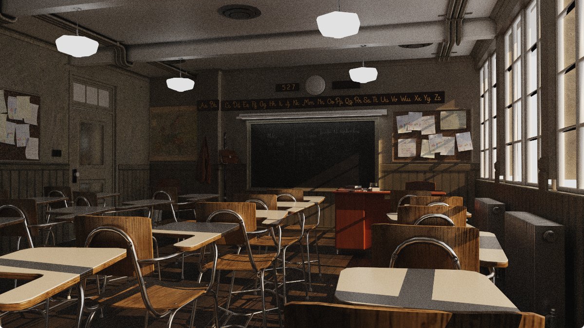
Cycles 参考

（Cycles不知道怎么回事，貌似弄错了BaseColor材质的color space）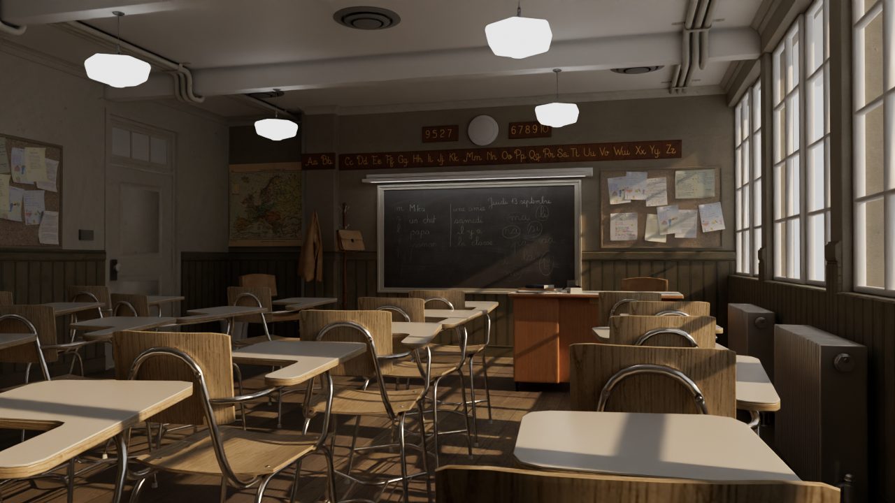

References

Real Time Rendering 4th Edition
Physically Based Rendering: From Theory To Implementation (PBRT)
Kanition PBRT v3 翻译版
Ray Tracing Gems 2
Google Filament - Energy loss in specular reflectance
glTF 2.0 Specification
Vulkan Specification - Shader Binding Table
RefractiveIndex.INFO
Sampling the GGX Distribution of Visible Normals - Heitz, E. (2018)
Understanding the Masking-Shadowing Function in Microfacet-Based BRDFs - Heitz, E. (2014)
Theory for Off-Specular Reflection From Roughened Surfaces - Torrance, K. E., & Sparrow, E. M. (1967)
Artist Friendly Metallic Fresnel - Gulbrandsen, O. (2014)
An Inexpensive BRDF Model for Physically-based Rendering - Schlick, C. (1994)
Multiple-Scattering Microfacet BSDFs with the Smith Model - Heitz, E., et al. (2016)
Revisiting Physically Based Shading at Imageworks - Kulla, C., & Conty, A. (2017)
Practical multiple scattering compensation for microfacet models - Turquin, E. (2019)
A Microfacet Based Coupled Specular-Matte BRDF Model with Importance Sampling - Kelemen, C., & Szirmay-Kalos, L. (2001)
nvpro-samples/vk_gltf_renderer
nvpro-samples/vk_mini_path_tracer
boksajak/referencePT
shader-slang/slangpy
Blender Source Code
Foundation/IBSDF.slang
Evermotion Archinteriors vol. 48
referencePT Bathroom Model

Preface#

准备工作#

SBT (Shader Binding Table) 及管线 API#

随机数生成及采样#

BxDF#

漫反射（朗伯反射）#

f/Eval#

Sample_f/Sample#

IBxDF 实现#

镜面反射（完美反射）#

f/Eval#

Sample_f/Sample#

IBxDF 实现#

Microfacet（微面）理论及建模#

VNDF#

重要性采样#

光泽反射 （Torrance-Sparrow）#

雅可比行列式#

f/Eval#

Sample_f/Sample#

反射与折射#

反射定律#

折射定律#

菲涅耳方程#

实数折射率#

复数折射率#

n,k 估计#

glTF 材质模型#

电介质模型#

导体模型#

fresnel_mix 的由来#

菲涅耳项估计#

能量守恒改进#

Random Walk (Heitz 2016)#

预积分查表（Kulla, Conty & Turquin）#

方向反照率 Albedo $E(w)$#

平均反射率 $F_{avg}$#

平均反照率 $E_{avg}$#

$E,E_{avg}$ 预积分#

Slang 写 Kernel？#

$f_{ms}$ 推导#

$f_{ms}$ 简化#

导体#

导体效果#

电介质#

电介质$E(\mu)$#

电介质效果#

总结#

样张#

Evermotion - Archinteriors vol. 48 - 008#

referencePT Bathroom#

Lumberyard Bistro#

Blender Classroom#

References#

Preface

准备工作

SBT (Shader Binding Table) 及管线 API

随机数生成及采样

BxDF

漫反射（朗伯反射）

f/Eval

Sample_f/Sample

IBxDF 实现

镜面反射（完美反射）

f/Eval

Sample_f/Sample

IBxDF 实现

Microfacet（微面）理论及建模

VNDF

重要性采样

光泽反射（Torrance-Sparrow）

雅可比行列式

f/Eval

Sample_f/Sample

反射与折射

反射定律

折射定律

菲涅耳方程

实数折射率

复数折射率

n,k 估计

glTF 材质模型

电介质模型

导体模型

fresnel_mix 的由来

菲涅耳项估计

能量守恒改进

Random Walk (Heitz 2016)

预积分查表（Kulla, Conty & Turquin）

方向反照率 Albedo $E(w)$

平均反射率 $F_{avg}$

平均反照率 $E_{avg}$

$E,E_{avg}$ 预积分

Slang 写 Kernel？

$f_{ms}$ 推导

$f_{ms}$ 简化

导体

导体效果

电介质

电介质$E(\mu)$

电介质效果

总结

样张

Evermotion - Archinteriors vol. 48 - 008

referencePT Bathroom

Lumberyard Bistro

Blender Classroom

References