Preface

参考主要来自 https://cp-algorithms.com/algebra/fft.html, https://en.wikipedia.org/wiki/Discrete_Fourier_transform, https://oi.wiki/math/poly/fft/

~~为照顾某OJ~~ 本文例程（杂项除外）C++标准仅需11；板子传送门,题目传送门

定义

多项式$A$的$DFT$即为$A$在各单位根$w_{n, k} = w_n^k = e^{\frac{2 k \pi i}{n}}$之值

$$ \begin{align} \text{DFT}(a_0, a_1, \dots, a_{n-1}) &= (y_0, y_1, \dots, y_{n-1}) \newline &= (A(w_{n, 0}), A(w_{n, 1}), \dots, A(w_{n, n-1})) \newline &= (A(w_n^0), A(w_n^1), \dots, A(w_n^{n-1})) \end{align} $$

$IDFT$ ($InverseDFT$) 即从这些值$(y_0, y_1, \dots, y_{n-1})$恢复多项式$A$的系数

$$ \text{IDFT}(y_0, y_1, \dots, y_{n-1}) = (a_0, a_1, \dots, a_{n-1}) $$

单位根有以下性质
- 积性 $$ w_n^n = 1 \newline w_n^{\frac{n}{2}} = -1 \newline w_n^k \ne 1, 0 \lt k \lt n $$
- 所有单位根和为$0$ $$ \sum_{k=0}^{n-1} w_n^k = 0 $$ 这点利用欧拉公式$e^{ix} = cos x + i\ sin x$看$n$边形对称性很显然

应用

考虑两个多项式$A, B$相乘 $$ (A \cdot B)(x) = A(x) \cdot B(x) $$

显然运用$DFT$可得

$$ DFT(A \cdot B) = DFT(A) \cdot DFT(B) $$

$A \cdot B$的系数易求

$$ A \cdot B = IDFT(DFT(A \cdot B)) = IDFT(DFT(A) \cdot DFT(B)) $$

逆操作（IDFT）

回忆$DFT$的定义 $$ \text{DFT}(a_0, a_1, \dots, a_{n-1}) = (A(w_n^0), A(w_n^1), \dots, A(w_n^{n-1})) $$

写成矩阵形式即为

$$ F = \begin{pmatrix} w_n^0 & w_n^0 & w_n^0 & w_n^0 & \cdots & w_n^0 \newline w_n^0 & w_n^1 & w_n^2 & w_n^3 & \cdots & w_n^{n-1} \newline w_n^0 & w_n^2 & w_n^4 & w_n^6 & \cdots & w_n^{2(n-1)} \newline w_n^0 & w_n^3 & w_n^6 & w_n^9 & \cdots & w_n^{3(n-1)} \newline \vdots & \vdots & \vdots & \vdots & \ddots & \vdots \newline w_n^0 & w_n^{n-1} & w_n^{2(n-1)} & w_n^{3(n-1)} & \cdots & w_n^{(n-1)(n-1)} \end{pmatrix} \newline $$

那么$DFT$操作即为

$$ F\begin{pmatrix} a_0 \newline a_1 \newline a_2 \newline a_3 \newline \vdots \newline a_{n-1} \end{pmatrix} = \begin{pmatrix} y_0 \newline y_1 \newline y_2 \newline y_3 \newline \vdots \newline y_{n-1} \end{pmatrix} $$

化简有

$$ y_k = \sum_{j=0}^{n-1} a_j w_n^{k j}, $$

其中范德蒙德阵$M$行列各项正交，可做出结论:

$$ F^{-1} = \frac{1}{n} F^\star, F_{i,j}^\star = \overline{F_{j,i}} $$

既有 $$ F^{-1} = \frac{1}{n} \begin{pmatrix} w_n^0 & w_n^0 & w_n^0 & w_n^0 & \cdots & w_n^0 \newline w_n^0 & w_n^{-1} & w_n^{-2} & w_n^{-3} & \cdots & w_n^{-(n-1)} \newline w_n^0 & w_n^{-2} & w_n^{-4} & w_n^{-6} & \cdots & w_n^{-2(n-1)} \newline w_n^0 & w_n^{-3} & w_n^{-6} & w_n^{-9} & \cdots & w_n^{-3(n-1)} \newline \vdots & \vdots & \vdots & \vdots & \ddots & \vdots \newline w_n^0 & w_n^{-(n-1)} & w_n^{-2(n-1)} & w_n^{-3(n-1)} & \cdots & w_n^{-(n-1)(n-1)} \end{pmatrix} $$

那么$IDFT$操作即为

$$ \begin{pmatrix} a_0 \newline a_1 \newline a_2 \newline a_3 \newline \vdots \newline a_{n-1} \end{pmatrix} = F^{-1} \begin{pmatrix} y_0 \newline y_1 \newline y_2 \newline y_3 \newline \vdots \newline y_{n-1} \end{pmatrix} $$

化简有

$$ a_k = \frac{1}{n} \sum_{j=0}^{n-1} y_j w_n^{-k j} $$

结论

注意到$w_i$使用共轭即为$n \cdot \text{IDFT}$
实现中稍作调整即可同时实现$DFT,IDFT$操作；接下来会用到

实现（FFT）

朴素包络时间复杂度为$O(n^2)$，这里不做阐述

$FFT$的过程如下

令 $A(x) = a_0 x^0 + a_1 x^1 + \dots + a_{n-1} x^{n-1}$, 按奇偶拆成两个子多项式

$$ \begin{align} A_0(x) &= a_0 x^0 + a_2 x^1 + \dots + a_{n-2} x^{\frac{n}{2}-1} \newline A_1(x) &= a_1 x^0 + a_3 x^1 + \dots + a_{n-1} x^{\frac{n}{2}-1} \end{align} $$

显然有

$$ A(x) = A_0(x^2) + x A_1(x^2). $$

设 $$ \left(y_k^0 \right)_{k=0}^{n/2-1} = \text{DFT}(A_0) $$

$$ \left(y_k^1 \right)_{k=0}^{n/2-1} = \text{DFT}(A_1) $$

$$ y_k = y_k^0 + w_n^k y_k^1, \quad k = 0 \dots \frac{n}{2} - 1. $$

对后半 $\frac{n}{2}$ 有

$$ \begin{align} y_{k+n/2} &= A\left(w_n^{k+n/2}\right) \newline &= A_0\left(w_n^{2k+n}\right) + w_n^{k + n/2} A_1\left(w_n^{2k+n}\right) \newline &= A_0\left(w_n^{2k} w_n^n\right) + w_n^k w_n^{n/2} A_1\left(w_n^{2k} w_n^n\right) \newline &= A_0\left(w_n^{2k}\right) - w_n^k A_1\left(w_n^{2k}\right) \newline &= y_k^0 - w_n^k y_k^1 \end{align} $$

即$y_{k+n/2} = y_k^0 - w_n^k y_k^1$，形式上非常接近$y_k$。综上：

$$ \begin{align} y_k &= y_k^0 + w_n^k y_k^1, &\quad k = 0 \dots \frac{n}{2} - 1, \newline y_{k+n/2} &= y_k^0 - w_n^k y_k^1, &\quad k = 0 \dots \frac{n}{2} - 1. \end{align} $$

该式即为所谓 “蝶形优化”

结论

很显然合并代价是$O(n)$；由$T_{\text{DFT}}(n) = 2 T_{\text{DFT}}\left(\frac{n}{2}\right) + O(n)$则知$FFT$可在$O(nlogn)$时间内解决问题
归并实现也将很简单

Code （归并）

又称 库利-图基演算法(Cooley-Tukey algorithm)；分治解决

若使用std::complex实现$w_n$可以直接用std::exp自带特化求得$w_n = e^{\frac{2\pi i}{n}}$
或者利用欧拉公式$e^{ix} = cos x + i\ sin x$可构造Complex w_n{ .real = cos(2 * PI / n), .imag = sin(2 * PI / n) }
结合之前所述的$DFT$, $IDFT$关系，使用$w_n = -e^{\frac{2\pi i}{n}}$并除$n$即求$IDFT$
时间复杂度$O(n\log n)$，由于对半分后归并，空间复杂度$O(n)$

void FFT(cvec& A, bool invert) {
    ll n = A.size(); 
    if (n == 1) return;
	cvec A0(n / 2), A1(n / 2);
	for (ll i = 0; i < n / 2; i++) 
        A0[i] = A[i * 2], A1[i] = A[i * 2 + 1];
  FFT(A0, invert), FFT(A1, invert);
  Complex w_n = exp(Complex{ 0, 2 * PI / n });
  if (invert) 
    w_n = conj(w_n);
  Complex w_k = Complex{ 1, 0 };
	for (ll k = 0; k < n / 2; k++) {
		A[k] = A0[k] + w_k * A1[k];
		A[k + n / 2] = A0[k] - w_k * A1[k];
    // 注意：除 log2(n) 次 2 即除 2^log2(n) = n
    if (invert) 
      A[k] /= 2, A[k + n / 2] /= 2;
		w_k *= w_n;
	}   
}
void FFT(cvec& a) { FFT(a, false); }
void IFFT(cvec& y) { FFT(y, true); }

Code （倍增）

归并法带来的额外空间其实可以优化掉——接下来介绍倍增法递推解决。

观察归并中最后回溯的顺序（以 $n=8$为例）
- 初始序列为 ${x_0, x_1, x_2, x_3, x_4, x_5, x_6, x_7}$
- 一次二分之后 ${x_0, x_2, x_4, x_6},{x_1, x_3, x_5, x_7 }$
- 两次二分之后 ${x_0,x_4} {x_2, x_6},{x_1, x_5},{x_3, x_7 }$
- 三次二分之后 ${x_0}{x_4}{x_2}{x_6}{x_1}{x_5}{x_3}{x_7 }$
注意力足够的话可以发现规律如下

In [17]: [int(bin(i)[2:].rjust(3,'0')[::-1],2) for i in range(8)]
Out[17]: [0, 4, 2, 6, 1, 5, 3, 7]

In [18]: [bin(i)[2:].rjust(3,'0')[::-1] for i in range(8)]
Out[18]: ['000', '100', '010', '110', '001', '101', '011', '111']

In [19]: [bin(i)[2:].rjust(3,'0') for i in range(8)]
Out[19]: ['000', '001', '010', '011', '100', '101', '110', '111']

即二进制倒序（对称），记该倒序为 $R(x)$

auto R = [n](ll x) {
    ll msb = ceil(log2(n)), res = 0;
    for (ll i = 0;i < msb;i++)
        if (x & (1 << i))
            res |= 1 << (msb - 1 - i);
    return res;
};

从下至上，以长度为$2,4,6,\cdots,n$递推，保持该顺序即可完成归并法所完成的任务
又因为对称，调整顺序也可在$O(n)$内完成；时间复杂度$O(n\log n)$，空间复杂度$O(1)$

void FFT(cvec& A, bool invert) {
    ll n = A.size();
    auto R = [n](ll x) {
        ll msb = ceil(log2(n)), res = 0;
        for (ll i = 0;i < msb;i++)
            if (x & (1 << i))
                res |= 1 << (msb - 1 - i);
        return res;
    };
    // Resort
    for (ll i = 0;i < n;i++)
        if (i < R(i))
            swap(A[i], A[R(i)]);
    // 从下至上n_i = 2, 4, 6,...,n直接递推
    for (ll n_i = 2;n_i <= n;n_i <<= 1) {
        Complex w_n = exp(Complex{ 0, 2 * PI / n_i });
        if (invert) w_n = conj(w_n);
        for (ll i = 0;i < n;i += n_i) {
            Complex w_k = Complex{ 1, 0 };
            for (ll j = 0;j < n_i / 2;j++) {
                Complex u = A[i + j], v = A[i + j + n_i / 2] * w_k;
                A[i + j] = u + v;
                A[i + j + n_i / 2] = u - v;
                if (invert)
                    A[i+j] /= 2, A[i+j+n_i/2] /= 2;
                w_k *= w_n;
            }
        }
    }
}
void FFT(cvec& a) { FFT(a, false); }
void IFFT(cvec& y) { FFT(y, true); }

数论变换（NTT）

虚数域内计算难免精度问题；数字越大误差越大且因为$exp$（或$sin, cos$）的使用极难修正。以下介绍数论变换（或快速数论变换）以允许在模数域下完成绝对正确的$O(nlogn)$包络。

在质数$p$, $F={\mathbb {Z}/p}$域下进行的DFT；注意到单位根的性质在模数下保留
同时显然的，有$$(w_n^m)^2 = w_n^n = 1 \pmod{p}, m = \frac{n}{2}$$；利用该性质我们可以利用快速幂求出$w_n^k$
当然，我们需要找到这样$g_n^n \equiv 1 \mod p$的$g$，使得$g_n$等效于$w_n$

原根

以下内容摘自：https://cp-algorithms.com/algebra/primitive-root.html#algorithm-for-finding-a-primitive-root,

定义：对任意$a$且存在$a$, $n$互质，且 $g^k \equiv a \mod n$，则称 $g$ 为模 $n$ 的原根。 结论：$n$的原根$g$,$g^k \equiv 1 \pmod n$， $k=\phi(n)$为$k$的最小解 下面介绍一种求原根的算法：

欧拉定义：若 $\gcd(a, n) = 1$，则 $a^{\phi(n)} \equiv 1 \pmod{n}$
对指数$p$, 朴素解法即为$O(n^2)$时间检查$g^d, d \in [0,\phi(n)] \not\equiv 1 \pmod n$
存在这样的$O(\log \phi (n) \cdot \log n)$解法：
- 找到$\phi(n)$因数$p_i \in P$，检查$g \in [1, n]$
- 对所有$p_i \in P$, $g ^ { \frac {\phi (n)} {p_i}} \not\equiv 1\pmod n $，此根即为一原根
证明请参见原文

#include "bits/stdc++.h"
using namespace std;
typedef long long ll; typedef vector<ll> vec; 
ll binpow_mod(ll a, ll b, ll m) {
    a %= m;
    ll res = 1;
    while (b > 0) {
        if (b & 1) res = (__int128)res * a % m;
        a = (__int128)a * a % m;
        b >>= 1;
    }
    return res;
}
ll min_primitive_root(ll p) {
    vec fac; ll phi = p - 1, n = phi;
    for (ll i = 2; i * i <= n; i++)
        if (n % i == 0) {
            fac.push_back(i);
            while (n % i == 0) n /= i;
        }
    if (n != 1) fac.push_back(n);
    for (ll r = 2; r <= p; r++) {
        bool ok = true;
        for (ll i = 0; ok && i < fac.size(); i++)
            ok &= binpow_mod(r, phi / fac[i], p) != 1;
        if (ok) return r;
    }
    return -1;
}
// min_primitive_root(754974721) = 11
// min_primitive_root(998244353) = 3
// min_primitive_root(7340033) = 3

实现（倍增）

综上，有质数$p$及其原根$g$对即可做到模数域下的单位根性质；常用的有 ($p=7 \times 17 \times 2^{23}+1=998244353, g=3$,$p=7 \times 2^{20} + 1 =7340033$)

这些数的欧拉函数满足$\phi(p) = p - 1 = c \times 2^k$形式，回忆欧拉函数$g^{p-1} \equiv 1 \pmod n$，很显然这很适合接下来我们要做的事情：遍历到长度$n_i$时，$w_{n_i} = e^{\frac{2\pi}{n_i}}$即等效于$g^{\frac{p-1}{n_i}}$。由于$n_i$ 倍增，$\frac{p-1}{n_i}$即为简单移位，同时整数除法也将无误差。

Code （倍增）

void NTT(vec& A, ll p, ll g, bool invert) {
  ll n = A.size();
  auto R = [n](ll x) {
      ll msb = ceil(log2(n)), res = 0;
      for (ll i = 0;i < msb;i++)
          if (x & (1 << i))
              res |= 1 << (msb - 1 - i);
      return res;
  };
  // Resort
  for (ll i = 0;i < n;i++)
      if (i < R(i)) swap(A[i], A[R(i)]);
  // 从下至上n_i = 2, 4, 6,...,n直接递推
  ll inv_2 = binpow_mod(2, p - 2, p);
  for (ll n_i = 2;n_i <= n;n_i <<= 1) {
      ll w_n = binpow_mod(g, (p - 1) / n_i, p);
      if (invert)
          w_n = binpow_mod(w_n, p - 2, p);
      for (ll i = 0;i < n;i += n_i) {
          ll w_k = 1;
          for (ll j = 0;j < n_i / 2;j++) {
              ll u = A[i + j], v = A[i + j + n_i / 2] * w_k;
              A[i + j] = (u + v + p) % p;
              A[i + j + n_i / 2] = (u - v + p) % p;
              if (invert) {
                  A[i + j] = A[i + j] * inv_2 % p;
                  A[i + j + n_i / 2] = A[i + j + n_i / 2] * inv_2 % p;
              }
              w_k = w_k * w_n % p;
          }
      }
  }
}
void FFT(vec& a) { NTT(a,998244353, 3, false); }
void IFFT(vec& y) { NTT(y, 998244353,3, true); }

余弦变换（DCT）

见下文实现；采用了以下$\text{DCT-II, DCT-III}$形式：

DCT-2 及其正则化系数

$$ y_k = 2f \sum_{n=0}^{N-1} x_n \cos\left(\frac{\pi k(2n+1)}{2N} \right) \newline \begin{split}f = \begin{cases} \sqrt{\frac{1}{4N}} & \text{if }k=0, \ \sqrt{\frac{1}{2N}} & \text{otherwise} \end{cases}\end{split} $$

DCT-3 $$ y_k = \frac{x_0}{\sqrt{N}} + \sqrt{\frac{2}{N}} \sum_{n=1}^{N-1} x_n \cos\left(\frac{\pi(2k+1)n}{2N}\right) $$

Reference (lib/poly.hpp)

本文所提及的$\text{DFT/FFT/(F)NTT}$魔术总结如下，开箱即用。

#include <span>
#include <cmath>
#include <vector>
#include <complex>
#include <numbers>
constexpr double PI = std::numbers::pi;
inline long long binpow_mod(long long a, long long b, long long m, long long res = 1) {
    for (a %= m; b; b >>= 1) res = (b & 1) ? (res * a % m) : res, a = a * a % m;
    return res;
};
inline bool is_pow2(const size_t x) { return (x & (x - 1)) == 0; }

enum class transform_result {
    SUCCESS = 0,
    INVALID_SIZE = 1,
    INVALID_INPUT = 2,
    INVALID_COEFFICIENT = 3,
};
template <typename T = size_t> struct bit_reversal {
    std::vector<T> bit;
    explicit bit_reversal(const size_t n) : bit(n) {
        for (size_t i = 0; i < n; i++) {
            bit[i] = bit[i >> 1] >> 1;
            if (i & 1) bit[i] |= (n >> 1);
        }
    }
    size_t operator[](size_t i) const { return bit[i]; }
};
template <typename Complex = std::complex<double>, bool Invert = false> struct FFT {
    using value_t = Complex;
    using span_t = std::span<value_t>;
    class twiddle_factor {
        std::vector<Complex> omega;
    public:
        explicit twiddle_factor(const size_t n) : omega(n) {
            // \sum_{i=1}^{\log_2 n} 2^{i - 1} = 2^{\log_2 n} - 1 = n - 1
            for (size_t n_i = 2, i = 1; n_i <= n; n_i <<= 1) {
                Complex w_n = std::exp(Complex{ 0, -2 * PI / n_i });
                if constexpr (Invert) w_n = std::conj(w_n);
                Complex w_k = Complex{ 1, 0 };
                for (size_t k_i = 0; k_i < n_i / 2; k_i++) {
                    omega[i++] = w_k;
                    w_k *= w_n;
                }
            }
        }
        Complex get(const size_t n_i, const size_t k_i) const { return omega[n_i / 2 + k_i]; }
        const size_t size() const { return omega.size(); }
    };
private:
    const twiddle_factor omega;
    const bit_reversal<> rev;
public:
    const size_t size;
    FFT(const size_t n) : omega(n), rev(n), size(n) {};
    transform_result operator()(span_t a) const {
        const size_t n = a.size();
        if (!is_pow2(n) || size != n) return transform_result::INVALID_SIZE;
        for (size_t i = 0, r; i < n; i++)
            if (i < (r = rev[i])) std::swap(a[i], a[r]);
        for (size_t n_i = 2; n_i <= n; n_i <<= 1) {
            for (size_t i = 0; i < n; i += n_i) {
                for (size_t j = 0; j < n_i / 2; j++) {
                    Complex u = a[i + j], v = a[i + j + n_i / 2] * omega.get(n_i, j);
                    a[i + j] = u + v;
                    a[i + j + n_i / 2] = u - v;
                    if constexpr (Invert) a[i + j] /= 2, a[i + j + n_i / 2] /= 2;
                }
            }
        }
        return transform_result::SUCCESS;
    }
};
template <typename Complex = std::complex<double>> using IFFT = FFT<Complex, true>;
template <typename Integer = long long, bool Invert = false> struct NTT {
    using value_t = Integer;
    using span_t = std::span<value_t>;
    class twiddle_factor {
        std::vector<Integer> omega;
    public:
        explicit twiddle_factor(const size_t n, const Integer p, const Integer g) : omega(n) {
            // \sum_{i=1}^{\log_2 n} 2^{i - 1} = 2^{\log_2 n} - 1 = n - 1
            for (size_t n_i = 2, i = 1; n_i <= n; n_i <<= 1) {
                Integer w_n = binpow_mod(g, (p - 1) / n_i, p);
                if constexpr (Invert) w_n = binpow_mod(w_n, p - 2, p);
                Integer w_k = 1;
                for (size_t k_i = 0; k_i < n_i / 2; k_i++) {
                    omega[i++] = w_k;
                    w_k = w_n * w_k % p;
                }
            }
        }
        Integer get(const size_t n_i, const size_t k_i) const { return omega[n_i / 2 + k_i]; }
        const size_t size() const { return omega.size(); }
    };
private:
    const twiddle_factor omega;
    const bit_reversal<> rev;
public:
    const Integer p, g, inv2;
    const size_t size;
    NTT(const size_t n, const Integer p, const Integer g)
        : omega(n, p, g), rev(n), size(n), p(p), g(g), inv2(binpow_mod(2, p - 2, p)) {};
    transform_result operator()(span_t a) const {
        const size_t n = a.size();
        if (!is_pow2(n) || size != n) return transform_result::INVALID_SIZE;
        for (size_t i = 0, r; i < n; i++)
            if (i < (r = rev[i])) std::swap(a[i], a[r]);
        for (size_t n_i = 2; n_i <= n; n_i <<= 1) {
            for (size_t i = 0; i < n; i += n_i) {
                Integer w_k = 1;
                for (size_t j = 0; j < n_i / 2; j++) {
                    Integer u = a[i + j], v = a[i + j + n_i / 2] * omega.get(n_i, j);
                    a[i + j] = (u + v + p) % p;
                    a[i + j + n_i / 2] = (u - v + p) % p;
                    if constexpr (Invert) {
                        a[i + j] = (a[i + j] * inv2 % p + p) % p;
                        a[i + j + n_i / 2] = (a[i + j + n_i / 2] * inv2 % p + p) % p;
                    }
                }
            }
        }
        return transform_result::SUCCESS;
    }
};
template <typename Integer = long long> using INTT = NTT<Integer, true>;
template <typename Real = double, typename DFT = FFT<>> struct DCT2 {
    using value_t = Real;
    using span_t = std::span<value_t>;
    using complex = typename DFT::value_t;
    using work_area_span_t = std::span<complex>;
private:
    DFT dft;
    std::vector<complex> work_area;
    std::vector<complex> omega;
public:
    const size_t size;
    DCT2(const size_t n, bool create_work_area = true) : dft(n * 2), omega(n), size(n) {
        for (size_t m = 0, N = 2 * n; m < n; m++) {
            Real w_ang = -PI * m / N;
            omega[m] = std::exp(complex{ 0, w_ang });
        }
        if (create_work_area) work_area.resize(n * 2);
    };
    transform_result operator()(span_t a, work_area_span_t work_area) const {
        // https://docs.scipy.org/doc/scipy/reference/generated/scipy.fftpack.dct.html
        // https://zh.wikipedia.org/wiki/离散余弦变换#方法一[8]
        const size_t n = a.size(), N = 2 * n;
        if (!is_pow2(n) || size != n || work_area.size() != N) return transform_result::INVALID_SIZE;
        for (size_t i = 0; i < n; i++) work_area[i] = work_area[N - i - 1] = a[i];
        dft(work_area);
        const Real k2N = std::sqrt(N), k4N = std::sqrt(2.0 * N);
        for (size_t m = 0; m < n; m++) {
            complex w_n = omega[m];
            a[m] = (work_area[m] * w_n).real(); // imag = 0
            a[m] /= (m == 0 ? k4N : k2N);
        }
        return transform_result::SUCCESS;
    }
    transform_result operator()(span_t a) { return operator()(a, work_area); }
};
template <typename Real = double, typename IDFT = IFFT<>> struct DCT3 {
    using value_t = Real;
    using span_t = std::span<value_t>;
    using complex = typename IDFT::value_t;
    using work_area_span_t = std::span<complex>;
private:
    IDFT idft;
    std::vector<complex> work_area;
    std::vector<complex> omega;
public:
    const size_t size;
    DCT3(const size_t n, bool create_work_area = true) : idft(n), size(n), omega(n) {
        for (size_t m = 0, N = 2 * n; m < n; m++) {
            Real w_ang = PI * m / N;
            omega[m] = std::exp(complex{ 0, w_ang });
        }
        if (create_work_area) work_area.resize(n);
    };
    transform_result operator()(span_t a, work_area_span_t work_area) const {
        // https://dsp.stackexchange.com/questions/51311/computation-of-the-inverse-dct-idct-using-dct-or-ifft
        // https://docs.scipy.org/doc/scipy/reference/generated/scipy.fftpack.dct.html
        const size_t n = a.size(), N = 2 * n;
        if (!is_pow2(n) || size != n || work_area.size() != n) return transform_result::INVALID_SIZE;
        for (size_t i = 0; i < n; i++) work_area[i] = a[i];
        a[0] /= std::sqrt(2.0);
        const Real k2N = std::sqrt(N);
        for (size_t m = 0; m < n; m++) {
            complex w_n = omega[m];
            work_area[m] = a[m] * k2N * w_n;
        }
        idft(work_area);
        for (size_t m = 0; m < n / 2; m++) {
            a[m * 2] = work_area[m].real();
            a[m * 2 + 1] = work_area[n - m - 1].real();
        }
        return transform_result::SUCCESS;
    }    
    transform_result operator()(span_t a) { return operator()(a, work_area); }
};

Problems

A * B

https://acm.hdu.edu.cn/showproblem.php?pid=1402
大整数乘法
$10$ 进制数，各位数字从低到高为$d_i$可看作是多项式$A(x) = x^n \times d_n + … + x^1 \times d_1 + x^0 \times d_0$于$x=10$时的解
两个十进制数即可看成是$A(x), B(x)$，求$A(x) * B(x)$即求$AB(x)$，由上文所述$\text{DFT,IDFT}$关系已知我们可以借此通过$\text{FFT}$在$O(n\log n)$时间计算这样的数
由于是$10$进制，最后多项式的系数即对应$x=10$解；注意进位。

void carry(Poly::IVec& a, ll radiax) {
    for (ll i = 0; i < a.size() - 1; i++)
        a[i + 1] += a[i] / radiax,
        a[i] %= radiax;
}
int main() {
    fast_io();
    /* El Psy Kongroo */
    string a, b;
    while (cin >> a >> b)
    {
        {
            Poly::IVec A(a.size()), B(b.size());
            for (ll i = 0; i < a.size(); i++)
                A[i] = a[a.size() - 1 - i] - '0';
            for (ll i = 0; i < b.size(); i++)
                B[i] = b[b.size() - 1 - i] - '0';
            ll len = Poly::conv::convolve(A, B);
            carry(A, 10u);
            for (ll i = len - 1, flag = 0; i >= 0; i--) {
                flag |= A[i] != 0;
                if (flag || i == 0)
                    cout << (ll)A[i];
            }
            cout << endl;
        }
    }
}

A + B 频率

https://open.kattis.com/problems/aplusb
给定整数序列$A$,$B$，求$a \in A, b \in B, a + b$的结果可能及数量
考虑这样转化成多项式问题：令 $ P_a(x) = \sum x^{A_i}, P_b(x) = \sum x^{B_i} $
给定例子$a = [1,~ 2,~ 3], b = [2,~ 4]$，这样构造的$P_aP_b$有 $$ (1 x^1 + 1 x^2 + 1 x^3) (1 x^2 + 1 x^4) = 1 x^3 + 1 x^4 + 2 x^5 + 1 x^6 + 1 x^7 $$
如此发现指数对应系数即各种可能数量

循环数乘

给定长$n$整数序列$A$,$B$，令$C_{p,i} = B_{(i + p) \mod n}$,求任意$A \cdot C_p$的值
回顾多项式相乘的系数即这样的包络 $$ c[k] = \sum_{i+j=k} a[i] b[j] $$
令$A$逆序，然后补$n$个$0$；令$B$补$B$本身
即$A_i = 0 (i \gt n - 1)$, 可见此时我们有

$$ c[k] = \sum_{i+j=k} a[i] b[j] = \sum_{i=0}^{n-1} a[i] b[k-i] $$

对$i + k > n$, $b[(i+k) % n] = b[i + k - n + 1]$；上式即为$p = k - n + 1$时结果
即$c[p + n - 1]$对应$p$时原$A \cdot C_p$值

字串匹配

给定字串$S$和模式串$P$，每个字符$C_i\in[0,26]$,统计$P$在$S$中出现总次数
- 构造多项式$A(x) = \sum a_i x^i$，其中$a_i = e^{\frac{2 \pi S_i}{26}}$
- 令$S$为其倒序，构造多项式$B(x)=\sum b_i x^i$,其中$b_i = e^{-\frac{2 \pi P_i}{26}}$
注意包络后

$$ c_{m-1+i} = \sum_{j = 0}^{m-1} a_{i+j} \cdot b_{m-1-j} = \sum_{j=0}^{m-1}e^{\frac{2 \pi S_{i+j} - 2\pi P_j}{26}} $$

显然若匹配则$e^{\frac{2 \pi S_{i+j} - 2\pi P_j}{26}} = e^0 = 1$，那么全部匹配当且仅当$c_{m-1+i} = m$，模式串$P$在$S_i$处有出现

附：部分匹配

设$P$中部分字符任意，则倒序后可令这些位置多项式系数$b_i=0$；设有$x$个这种位置
回顾上式易知当且仅当匹配到这些系数时有$c_i = \sum_{j=0}^{m-1-x} e^{\cdots} + \sum_0^x 0$
显然，当$c_{m-1+i} = m - x$，带任意匹配模式的模式串$P$在$S_i$处有出现

图像处理？？？

正常人应该用FFTW - 但可惜你是ACM选手。

lib/image.hpp

STB is All You Need.

#pragma once
#ifndef _POLY_HPP
#include "poly.hpp"
#endif
#define _IMAGE_HPP
#define STB_IMAGE_IMPLEMENTATION
#define STB_IMAGE_WRITE_IMPLEMENTATION
#include "stb/stb_image.h"
#include "stb/stb_image_write.h"
namespace Image {
using Texel = unsigned char;
using Image = std::vector<Poly::RVec2>;
using Poly::ll, Poly::lf;
// Channels, Height, Width
inline std::tuple<ll, ll, ll> image_size(const Image& img) {
    if (!img.size()) return { 0, 0, 0 };    
    auto [h, w] = Poly::utils::size_of(img[0]);    
    return { img.size(), h, w };
}
// Assuming 8bit sRGB space
template <typename Texel> Image from_texels(const Texel* img_data, int w, int h, int nchn) {
    Image chns(nchn, Poly::RVec2(h, Poly::RVec(w)));
    for (ll y = 0; y < h; ++y)
        for (ll x = 0; x < w; ++x)
            for (ll c = 0; c < nchn; ++c) chns[c][y][x] = img_data[(y * w + x) * nchn + c];
    return chns;
}
vector<Texel> to_texels(const Image& res, int& w, int& h, int& nchn) {
    std::tie(nchn, h, w) = image_size(res);
    vector<Texel> texels(w * h * nchn);
    for (ll y = 0; y < h; ++y)
        for (ll x = 0; x < w; ++x)
            for (ll c = 0; c < nchn; ++c) {
                ll t = std::round(res[c][y][x]);
                texels[(y * w + x) * nchn + c] = max(min(255ll, t), 0ll);
            }
    return texels;
}
inline Image from_file(const char* filename, bool hdr = false) {
    int w, h, nchn;
    Texel* img_data = stbi_load(filename, &w, &h, &nchn, 0);
    assert(img_data && "cannot load image");
    auto chns = from_texels(img_data, w, h, nchn);
    stbi_image_free(img_data);
    return chns;
}
inline void to_file(const Image& res, const char* filename, bool hdr = false) {
    int w, h, nchn;
    auto texels = to_texels(res, w, h, nchn);
    int success = stbi_write_png(filename, w, h, nchn, texels.data(), w * nchn);
    assert(success && "image data failed to save!");
}
inline Image create(int nchn, int h, int w, lf fill) {
    Image image(nchn);
    for (auto& ch : image) Poly::utils::resize(ch, { h, w }, fill);
    return image;
}
inline Poly::RVec2& to_grayscale(Image& image) {
    auto [nchn, h, w] = image_size(image);
    auto& ch0 = image[0];
    // L = R * 299/1000 + G * 587/1000 + B * 114/1000
    for (ll c = 0; c < nchn; c++) {
        for (ll i = 0; i < h; i++) {
            for (ll j = 0; j < w; j++) {
                if (c == 0 && nchn != 1) ch0[i][j] *= 0.299;
                if (c == 1) ch0[i][j] += image[1][i][j] * 0.587;
                if (c == 2) ch0[i][j] += image[2][i][j] * 0.144;
            }
        }
    }
    return ch0;
}
} // namespace Image

二维包络

想玩转超大kernel还想不等半年？？

设原图像$A[N,M]$,包络核$B[K,L]$空间上进行包络有时间复杂度$O(N * M * K * L)$
利用$\text{FFT}$则为$O(N * M * log(N * M))$

高斯模糊

#include "bits/stdc++.h"
using namespace std;
typedef long long ll; typedef double lf; typedef pair<ll, ll> II; typedef vector<ll> vec;
const inline void fast_io() { ios_base::sync_with_stdio(false); cin.tie(0u); cout.tie(0u); }
const lf PI = acos(-1);

#include "lib/poly.hpp"
#include "lib/image.hpp"
Poly::RVec2 gaussian(ll size, lf sigma) {
    Poly::RVec2 kern(size, Poly::RVec(size));
    lf sum = 0.0;
    ll x0y0 = size / 2;
    lf sigma_sq = sigma * sigma;
    lf term1 = 1.0 / (2.0 * PI * sigma_sq);
    for (ll i = 0; i < size; ++i) {
        for (ll j = 0; j < size; ++j) {
            ll x = i - x0y0, y = j - x0y0;
            lf term2 = exp(-(lf)(x * x + y * y) / (2.0 * sigma_sq));
            kern[i][j] = term1 * term2;
            sum += kern[i][j];
        }
    }
    for (ll i = 0; i < size; ++i)
        for (ll j = 0; j < size; ++j)
            kern[i][j] /= sum;
    return kern;
}
const auto __Exec = std::execution::par_unseq;
int main() {
    const char* input = "data/input.png";
    const char* output = "data/output.png";
    const int kern_size = 25;
    const lf kern_sigma = 7.0;

    Poly::RVec2 kern = gaussian(kern_size, kern_sigma);
    auto image = Image::from_file(input);
    {
        auto [nchn,h,w] = Image::image_size(image);
        cout << "preparing image w=" << w << " h=" << h << " nchn=" << nchn << endl;
        for_each(__Exec, image.begin(), image.end(), [&](auto& ch) {
            cout << "channel 0x" << hex << &ch << dec << endl;
            auto c_ch = Poly::utils::as_complex(ch), k_ch = Poly::utils::as_complex(kern);
            Poly::conv::convolve2D(c_ch, k_ch, __Exec);
            ch = Poly::utils::as_real(c_ch);
        });
    }
    {
        Image::to_file(image, output);
        auto [nchn,h,w] = Image::image_size(image);
        cout << "output image w=" << w << " h=" << h << " nchn=" << nchn << endl;
    }
    return 0;
}

测试样例
输入输出

Wiener 去卷积（逆包络）

2025，Codeforces 4.1 H题见

https://en.wikipedia.org/wiki/Wiener_deconvolution
Wiener 去卷积可表示为

$$ \ F(f) = \frac{H^\star(f)}{ |H(f)|^2 + N(f) }G(f)= \frac{H^\star(f)}{ H(f)\times H^\star(f) + N(f) }G(f) $$

都在频域下，其中$F$为原图像，$G$为包络后图像，$H$为卷积核，$N$为噪声函数

#include "bits/stdc++.h"
using namespace std;
typedef long long ll; typedef double lf; typedef pair<ll, ll> II; typedef vector<ll> vec;
const inline void fast_io() { ios_base::sync_with_stdio(false); cin.tie(0u); cout.tie(0u); }
const lf PI = acos(-1);

#include "lib/poly.hpp"
#include "lib/image.hpp"
Poly::RVec2 gaussian(ll size, lf sigma) {
	Poly::RVec2 kern(size, Poly::RVec(size));
	lf sum = 0.0;
	ll x0y0 = size / 2;
	lf sigma_sq = sigma * sigma;
	lf term1 = 1.0 / (2.0 * PI * sigma_sq);
	for (ll i = 0; i < size; ++i) {
		for (ll j = 0; j < size; ++j) {
			ll x = i - x0y0, y = j - x0y0;
			lf term2 = exp(-(lf)(x * x + y * y) / (2.0 * sigma_sq));
			kern[i][j] = term1 * term2;
			sum += kern[i][j];
		}
	}
	for (ll i = 0; i < size; ++i)
		for (ll j = 0; j < size; ++j)
			kern[i][j] /= sum;
	return kern;
}
const auto exec = std::execution::par_unseq;
int main() {
    const char* input = "data/blurred.png";
    const char* output = "data/deblur.png";
    const int kern_size = 25;
    const lf kern_sigma = 7.0;

    Poly::RVec2 kern = gaussian(kern_size, kern_sigma);
    auto wiener = [&](Poly::RVec2& ch, Poly::RVec2 kern, lf noise = 5e-6) {
        II og_size = { ch.size(), ch[0].size() };
        II size = Poly::utils::to_pow2({ ch.size(), ch[0].size() }, { kern.size(), kern[0].size() });
        auto [N, M] = size;
        Poly::utils::resize(ch, size, 255.0);
        // 需要窗口
        Poly::CVec2 img_fft = Poly::utils::as_complex(ch);
        ch = Poly::utils::as_real(img_fft);
        Poly::transform::DFT2(img_fft, exec);
        Poly::CVec2 kern_fft = Poly::utils::as_complex(kern);
        Poly::utils::resize(kern_fft, size);
        Poly::transform::DFT2(kern_fft, exec);
        for (ll i = 0; i < N; i++)
            for (ll j = 0; j < M; j++) {
                auto kern_fft_conj = conj(kern_fft[i][j]);
                auto denom = kern_fft[i][j] * kern_fft_conj + noise;
                img_fft[i][j] = (img_fft[i][j] * kern_fft_conj) / denom;
            }
        Poly::transform::IDFT2(img_fft, exec);
        ch = Poly::utils::as_real(img_fft);
        Poly::utils::resize(ch, og_size);
    };
    auto image = Image::from_file(input);
    {
        auto [nchn,h,w] = Image::image_size(image);
        cout << "preparing image w=" << w << " h=" << h << " nchn=" << nchn << endl;
        for_each(exec, image.begin(), image.end(), [&](auto& ch) {
            cout << "channel 0x" << hex << &ch << dec << endl;
            wiener(ch, kern);
        });
    }
    {
        Image::to_file(image, output);
        auto [nchn,h,w] = Image::image_size(image);
        cout << "output image w=" << w << " h=" << h << " nchn=" << nchn << endl;
    }
    return 0;
}

测试样例
输入输出

图像压缩（DCT）

JPEG格式采用的即为$8\times8$ DCT块变换，丢掉高频信息（频域$u,v$大位置）后量化存储

这里演示一种naive的压缩方式，和MATLAB所述图像压缩样例一致，以下面矩阵掩盖系数： $$ \text{mask} = \begin{bmatrix} 1 & 1 & 1 & 1 & 0 & 0 & 0 & 0 \newline 1 & 1 & 1 & 0 & 0 & 0 & 0 & 0 \newline 1 & 1 & 0 & 0 & 0 & 0 & 0 & 0 \newline 1 & 0 & 0 & 0 & 0 & 0 & 0 & 0 \newline 0 & 0 & 0 & 0 & 0 & 0 & 0 & 0 \newline 0 & 0 & 0 & 0 & 0 & 0 & 0 & 0 \newline 0 & 0 & 0 & 0 & 0 & 0 & 0 & 0 \newline 0 & 0 & 0 & 0 & 0 & 0 & 0 & 0 \newline \end{bmatrix} $$

#include "bits/stdc++.h"
using namespace std;
typedef long long ll;typedef double lf;typedef pair<ll, ll> II; typedef vector<ll> vec;
const lf PI = acos(-1);
#include "lib/image.hpp"
#include "lib/poly.hpp"
auto block8x8 = [](auto&& op, auto& src) { return Poly::block::block2D(op, src, 8, 8, std::execution::par_unseq); };
int main() {
    /* image to dct */
    auto image = Image::from_file("data/cameraman.png");
    auto& source = Image::to_grayscale(image);
    auto [nchn, h, w] = Image::image_size(image);
    Poly::utils::resize(source, { Poly::utils::to_pow2(h), Poly::utils::to_pow2(w) });
    cout << "Processing..." << w << "x" << h << endl;
    block8x8([](Poly::RVec2& rect) { Poly::transform::DCT2(rect, execution::seq); }, source);
    cout << "Saving." << endl;
    Image::to_file(Image::Image{ source }, "data/dct.png");
    cout << "Dropping coefficents." << endl;
    block8x8(
        [](Poly::RVec2& rect) {
            auto [n, m] = Poly::utils::size_of(rect);
            for (ll i = 0; i < n; i++) for (ll j = 0; j < m; j++)
                if (i >= 4 || j >= (n / 2 - i)) rect[i][j] = 0;
        },
        source);
    Image::to_file(Image::Image{ source }, "data/dct_dropped.png");
    cout << "Restoring." << endl;
    block8x8([](Poly::RVec2& rect) { Poly::transform::IDCT2(rect, execution::seq); }, source);
    cout << "Saving." << endl;
    Image::to_file(Image::Image{ source }, "data/idct.png");
    return 0;
}

输入	DCT	丢掉三角阵的DCT	IDCT

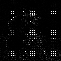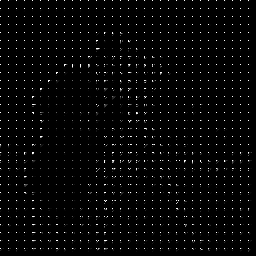Preface#

定义#

应用#

逆操作（IDFT）#

结论#

实现（FFT）#

结论#

Code （归并）#

Code （倍增）#

数论变换 （NTT）#

原根#

实现（倍增）#

Code （倍增）#

余弦变换（DCT）#

Reference (lib/poly.hpp)#

Problems#

A * B#

A + B 频率#

循环数乘#

字串匹配#

附：部分匹配#

图像处理？？？#

lib/image.hpp#

二维包络#

高斯模糊#

Wiener 去卷积（逆包络）#

图像压缩 （DCT）#

Preface

定义

应用

逆操作（IDFT）

结论

实现（FFT）

结论

Code （归并）

Code （倍增）

数论变换（NTT）

原根

实现（倍增）

Code （倍增）

余弦变换（DCT）

Reference (lib/poly.hpp)

Problems

A * B

A + B 频率

循环数乘

字串匹配

附：部分匹配

图像处理？？？

lib/image.hpp

二维包络

高斯模糊

Wiener 去卷积（逆包络）

图像压缩（DCT）